3-D Dual-Tree Wavelet Transform

Compared to the separable DWT, the dual-tree DWT may provide even more improvement for 3D data processing than it does for 2D image processing. This is because in higher dimensions, the checkerboard artifact of the separable DWT becomes more severe. However, in higher dimensions the dual-tree DWT becomes even more expansive.

As in the 2D case, there are two versions of the 3D dual-tree wavelet transform: the real 3D dual-tree DWT is 4-times expansive, while the complex 3D dual-tree DWT is 8-times expansive. For both types of transform, each wavelet is oriented in a specific direction. For the 8-times expansive complex 3D dual-tree DWT, there are two wavelets in each orientation.

1. Real 3D Dual-tree Wavelet Transform

The real 3D dual-tree DWT of a data set x is implemented using four critically-sampled separable 3D DWTs in parallel. Then the subbands of the four DWTs are combined appropriately.

The following program, dualtree3D.m, computes the J-scale real 3D dual-tree DWT of a data set x.

function w = dualtree3D(x, J, Faf, af)

% 3D Dual-Tree Discrete Wavelet Transform
%
% USAGE:
%   w = dualtree3D(x, J, Faf, af)
% INPUT:
%   x - 3-D array
%   J - number of stages
%   Faf - first stage filters
%   af - filters for remaining stages
% OUPUT:
%   w{j}{i}{d} - wavelet coefficients
%        j = 1..J, i = 1..4, d = 1..7
%   w{J+1}{i} - lowpass coefficients
%        i = 1..4

% normalization
x = x/2;

M = [
    1 1 1
    2 2 1
    2 1 2
    1 2 2
];

for i = 1:4
    f1 = M(i,1);
    f2 = M(i,2);
    f3 = M(i,3);
    [xi w{1}{i}] = afb3D(x, Faf{f1}, Faf{f2}, Faf{f3});
    for k = 2:J
        [xi w{k}{i}] = afb3D(xi, af{f1}, af{f2}, af{f3});
    end
    w{J+1}{i} = xi;
end

for k = 1:J
    for m = 1:7
        [w{k}{1}{m} w{k}{2}{m} w{k}{3}{m} w{k}{4}{m}] = ...
            pm4(w{k}{1}{m}, w{k}{2}{m}, w{k}{3}{m}, w{k}{4}{m});
    end
end

The wavelet coefficients w are stored as a cell array. For j = 1..J, k = 1..4, d = 1..7, w{j}{k}{d} are the wavelet coefficients produced at scale j and orientation (k,d). The image x is recovered from w using the inverse transform, implemented by idualtree3D.m. The perfect reconstruction property of the transform is illustrated in the following code fragment.

>> x = rand(64,64,64);
>> J = 3;
>> [Faf, Fsf] = FSfarras;
>> [af, sf] = dualfilt1;
>> w = dualtree3D(x, J, Faf, af);
>> y = idualtree3D(w, J, Fsf, sf);
>> err = x - y;
>> max(max(max(abs(err))))

ans =

  3.7805e-008
  

There are 28 wavelets associated with the real 3D dual-tree DWT. The isosurface of one of the wavelets is shown in the following figure.

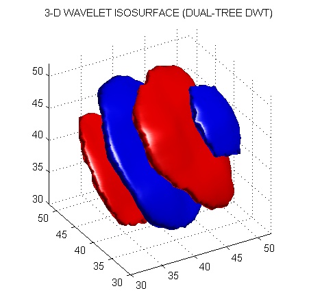
In contrast with the critically-sampled separable 3D DWT, the wavelet is free of checkerboard artifact. Each subband of the real 3D dual-tree DWT corresponds to a specific orientation. This figure was produced with the following Matlab program (dualtree3D_plots.m).

% dualtree3D_plots
% DISPLAY 3D WAVELETS OF DUALTREE3D.M

[Faf, Fsf] = FSfarras;
[af, sf] = dualfilt1;
J = 4;
L = 3*2^(J+1);
N = L/2^J;
x = zeros(L,L,L);
w = dualtree3D(x, J, Faf, af);
w{J}{4}{7}(N/2,N/2,N/2) = 1;
y = idualtree3D(w, J, Fsf, sf);
figure(1)
clf
v = 1:L;
S = 0.0025;
p1 = patch(isosurface(v,v,v,y,S));
isonormals(v,v,v,y,p1);
set(p1,'FaceColor','red','EdgeColor','none'); 
hold on
p2 = patch(isosurface(v,v,v,y,-S));
isonormals(v,v,v,y,p2);
set(p2,'FaceColor','blue','EdgeColor','none'); 
hold off
daspect([1 1 1]);
view(-30,30); 
camlight;
lighting phong
grid
axis([32 48 32 48 32 48])
set(gca,'fontsize',7)
title('3-D WAVELET ISOSURFACE (DUALTREE TRANSFORM)')
set(gcf,'paperposition',[0.5 0.5 0 0]+[0 0 4 3])
print -djpeg95 dualtree3D_plots

2. Complex 3-D Dual-tree Wavelet Transform

The complex 3D dual-tree DWT also gives rise to twice as many wavelets as the real 3D dual-tree DWT. The two wavelets in each orientation, can be interpreted as the real and imaginary parts of a complex-valued 3D wavelet. The complex 3D dual-tree is implemented as eight critically-sampled separable 3D DWTs operating in parallel. However, different filter sets are used in each of the three dimensions.

The complex 3D dual-tree DWT of an data set x is computed by the function, cplxdual3D.m.

function w = cplxdual3D(x, J, Faf, af)

% 3D Complex Dual-Tree Discrete Wavelet Transform
%
% w = cplxdual3D(x, J, Faf, af)
% INPUT:
%    x   - 3-D signal
%    J   - number of stages
%    Faf - first stage filters
%    af  - filters for remaining stages
% OUPUT:
%    w{j}{m}{n}{p}{d} - wavelet coefficients
%       j = 1..J, m = 1..2, n = 1..2, p = 1..2, d = 1..7
%    w{J+1}{m}{n}{d} - lowpass coefficients
%       m = 1..2, n = 1..2, p = 1..2, d = 1..7

for m = 1:2
    for n = 1:2
        for p = 1:2
            [lo w{1}{m}{n}{p}] = afb3D(x, Faf{m}, Faf{n}, Faf{p});
            for j = 2:J
                [lo w{j}{m}{n}{p}] = afb3D(lo, af{m}, af{n}, af{p});
            end
            w{J+1}{m}{n}{p} = lo;
        end
    end
end

for j = 1:J
    for m = 1:7
[w{j}{1}{1}{1}{m} w{j}{2}{2}{1}{m} w{j}{2}{1}{2}{m} w{j}{1}{2}{2}{m}] 
= ...
pm4(w{j}{1}{1}{1}{m}, w{j}{2}{2}{1}{m}, w{j}{2}{1}{2}{m}, 
w{j}{1}{2}{2}{m});

[w{j}{2}{2}{2}{m} w{j}{1}{1}{2}{m} w{j}{1}{2}{1}{m} w{j}{2}{1}{1}{m}] 
= ...
pm4(w{j}{2}{2}{2}{m}, w{j}{1}{1}{2}{m}, w{j}{1}{2}{1}{m}, 
w{j}{2}{1}{1}{m});
    end
end

The wavelet coefficients w are stored as a cell array. For j = 1..J, m = 1..2, n = 1..2, p = 1..2, d = 1..7, w{j}{m}{n}{p}{d} are the wavelet coefficients produced at scale j and orientation (m,n,d). With p = 1 we get the real part, with p = 2 we get the imaginary part. The function icplxdual3D.m computes the inverse transform.

The perfect reconstruction property of the transform is illustrated in the following code fragment.

>> x = rand(64,64,64);
>> J = 3;
>> [Faf, Fsf] = FSfarras;
>> [af, sf] = dualfilt1;
>> w = cplxdual3D(x, J, Faf, af);
>> y = icplxdual3D(w, J, Fsf, sf);
>> err = x - y;
>> max(max(max(abs(err))))

ans =

  3.7576e-008
  

The wavelets of the complex 3D dual-tree DWT are similar to those of the real 3D dual-tree DWT, however, there are two of them in each orientation. They can be interpreted as the real and imaginary parts of a complex-valued 3D wavelet. The following figures illustrate the isosurfaces of the real part, imaginary part, and magnitude of a complex-valued wavelet.

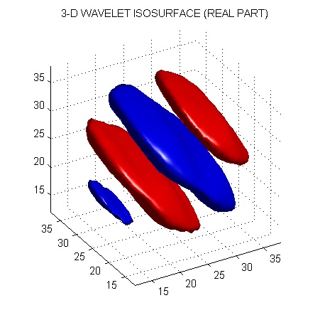
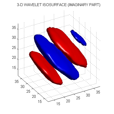
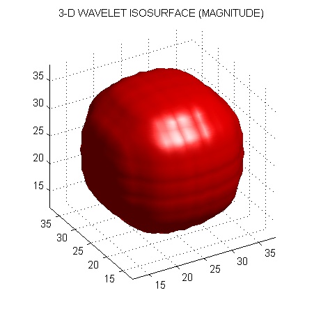
This figure was produced with the Matlab program, cplxdual3D_plots.m.

Summary of programs:

1. dualtree3D.m - Wavelet transform (real part)
2. idualtree3D.m - Inverse wavelet xform (real part)
3. dualtree3D_plots.m - Display wavelets (real part)
4. cplxdual3D.m - Complex wavelet xform
5. icplxdual3D.m - Inverse complex wavelet xform
6. cplxdual3D_plots.m - Display complex wavelets