Bivariate Shrinkage Functions for Wavelet Based Denoising

We have proposed a new simple non-Gaussian bivariate probability distribution function to model the statistics of wavelet coefficients of natural images. The model captures the dependence between a wavelet coefficient and its parent. Using Bayesian estimation theory we derive from this model a simple non-linear shrinkage function for wavelet denoising, which generalizes the soft thresholding approach of Donoho and Johnstone. The new shrinkage function, which depends on both the coefficient and its parent, yields improved results for wavelet-based image denoising.
Let w2 represent the parent of w1 (w2 is the wavelet coefficient at the same spatial position as w1, but at the next coarser scale). Then

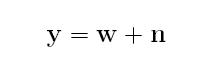
where w = (w1,w2), y = (y1,y2) and n = (n1,n2). The noise values n1, n2 are iid zero-mean Gaussian with variance \sigma_n^2. Based on the empirical histograms we have computed, we propose the following non-Gaussian bivariate pdf

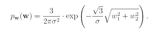
With this pdf, w1 and w2 are uncorrelated, but not independent. The MAP estimator of w1 yields the following bivariate shrinkage function

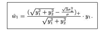
For this bivariate shrinkage function, the smaller the parent value, the greater the shrinkage. This is consistent with other models, but here it is derived using a Bayesian estimation approach beginning with the new bivariate non-Gaussian model. The plot is illustrated in the figure below.

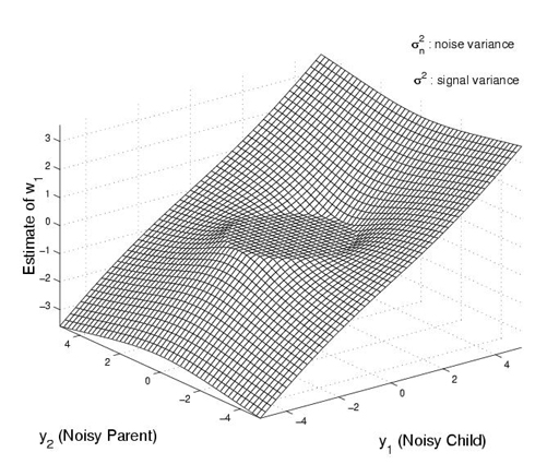
Fig. 2.1 A bivariate shrinkage function.

This bivariate shrinkage function can be implemented as the matlab function bishrink.m as follows

function [w1] = bishrink(y1,y2,T)
% Bivariate Shrinkage Function
% Usage :
%      [w1] = bishrink(y1,y2,T)
% INPUT :
%      y1 - a noisy coefficient value
%      y2 - the corresponding parent value
%      T  - threshold value
% OUTPUT :
%      w1 - the denoised coefficient

R  = sqrt(abs(y1).^2 + abs(y2).^2);
R = R - T;
R  = R .* (R > 0);
w1 = y1 .* R./(R+T); 

2. Local Adaptive Image Denoising

Using the bivariate shrinkage function above, we developed an effective and low complexity locally adaptive image denoising algorithm in [2]. This shrinkage function requires the prior knowledge of the noise variance and and the signal variance for each wavelet coefficient. Therefore the algorithm first estimates these parameters (see [2] for the recipe of the estimation rules).

Briefly, the algorithm is summarized as follows:

1. Calculate the noise variance.
2. For each wavelet coefficient,
   1. Calculate signal variance,
   2. Estimate each coefficient using the bivariate shrinkage function.

The following sections describe the implemetation of this algorithm using both the seperable DWT and the complex dual-tree DWT. (Necessary programs are provided).

2.1 Matlab implementation of wavelet-based denoising using the separable DWT

2.2 Matlab implementation of wavelet-based denoising using the dual-tree DWT

3. Examples:

Original Image View full size image	Noisy Image View full size image
Denoised Image (Seperable DWT) View full size image	Denoised Image (Dual-tree DWT) View full size image

4. References:

[1] : L. Sendur, I.W. Selesnick, "Bivariate shrinkage functions for wavelet-based denoising exploiting interscale dependency", IEEE Transactions on Signal Processing, 50(11), 2744-2756, Nov 2002.

[2] : L. Sendur, I.W. Selesnick, "Bivariate shrinkage with local variance estimation", IEEE Signal Processing Letters, 9(12), 438-441, Dec 2002.

[3] : L. Sendur, I.W. Selesnick, "A bivariate shrinkage function for wavelet-based denoising", IEEE International Conference on Acoustics, Speech, and Signal Processing, 2002.

[4] : L. Sendur, I.W. Selesnick, "Subband adaptive image denoising via bivariate shrinkage", IEEE International Conference on Image Processing (ICIP), 2002.