2-D Discrete Wavelet Transform

1. 2-D Filter Banks

To use the wavelet transform for image processing we must implement a 2D version of the analysis and synthesis filter banks. In the 2D case, the 1D analysis filter bank is first applied to the columns of the image and then applied to the rows. If the image has N1 rows and N2 columns, then after applying the 1D analysis filter bank to each column we have two subband images, each having N1/2 rows and N2 columns; after applying the 1D analysis filter bank to each row of both of the two subband images, we have four subband images, each having N1/2 rows and N2/2 columns. This is illustrated in the diagram below. The 2D synthesis filter bank combines the four subband images to obtain the original image of size N1 by N2.

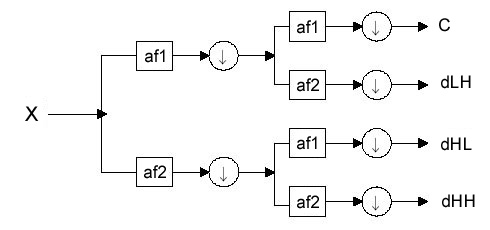
Fig. 2.1 One stage in multi-resolution wavelet decomposition of an image [3]

The 2D analysis filter bank is implemented with the Matlab function afb2D.m. This function calls a sub-function, afb2D_A.m, which applies the 1D analysis filter bank along one dimension only (either along the columns or along the rows). The function afb2D.m returns two variables: lo is the lowpass subband image; hi is a cell array containing the 3 other subband images.

function [lo, hi] = afb2D(x, af1, af2)

% 2D Analysis Filter Bank
%
% [lo, hi] = afb2D(x, af1, af2);
% INPUT:
%    x - NxM matrix, where min(N,M) > 2*length(filter)
%           (N, M are even)
%    af1 - analysis filter for the columns
%    af2 - analysis filter for the rows
%    afi(:, 1) - lowpass filter
%    afi(:, 2) - highpass filter
% OUTPUT:
%     lo, hi - lowpass, highpass subbands
%     hi{1} = 'lohi' subband
%     hi{2} = 'hilo' subband
%     hi{3} = 'hihi' subband

if nargin < 3
   af2 = af1;
end

% filter along columns
[L, H] = afb2D_A(x, af1, 1);

% filter along rows
[lo    hi{1}] = afb2D_A(L, af2, 2);
[hi{2} hi{3}] = afb2D_A(H, af2, 2);

The 2D synthesis filter bank is similarly implemented with the commands sfb2D.m and sfb2D_A.m.

2. 2D Discrete Wavelet Transform

As in the 1D case, the 2D discrete wavelet transform of a signal x is implemented by iterating the 2D analysis filter bank on the lowpass subband image. In this case, at each scale there are three subbands instead of one. The function, dwt2D.m, computes the J-scale 2D DWT w of an image x by repeatedly calling afb2D.m.

function w = dwt2D(x, J, af)

% discrete 2-D wavelet transform
%
% w = dwt2D(x, stages, af)
% INPUT:
%    x : NxM matrix (N, M even)
%    J : number of stages
%    af : analysis filters
% OUPUT:
%    w : cell array of wavelet coefficients

for k = 1:J
    [x w{k}] = afb2D(x, af, af);
end
w{J+1} = x; 

Again, w is a Matlab cell array;for j = 1..J, d = 1..3, w{j}{d} is one of the three subband images produced at stage j. w{J+1} is the lowpass subband image produced at the last stage. The function idwt2D.m computes the inverse 2D DWT.

The perfect reconstruction of the 2D DWT is verified in the following example. We create a random input signal x of size 128 by 64, apply the DWT and its inverse, and show it reconstructs x from the wavelet coefficients in w.

EXAMPLE (VERIFY PERFECT RECONSTRUNCTION) >> [af, sf] = farras; >> x = rand(128,64); >> w = dwt2D(x,3,af); >> y = idwt2D(w,3,sf); >> err = x-y; >> max(max(abs(err))) ans = 8.9817e-014

There are three wavelets associated with the 2D wavelet transform. The following figure illustrates three wavelets as gray scale images.

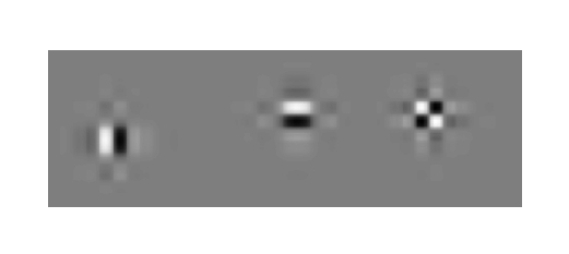
Note that the first two wavelets are oriented in the vertical and horizontal directions, however, the third wavelet does not have a dominant orientation. The third wavelet mixes two diagonal orientations, which gives rise to the checkerboard artifact. (The 2D DWT is poor at isolating the two diagonal orientations.) This figure was produced with the following Matlab code fragment (dwt2D_plots.m).

% dwt2D_plots
% DISPLAY 2D WAVELETS OF DWT2D.M

[af, sf] = farras;
J = 5;                      
L = 3*2^(J+1);
N = L/2^J;
x = zeros(L,3*L);
w = dwt2D(x,J,af);
w{J}{1}(N/2,N/2+0*N) = 1;
w{J}{2}(N/2,N/2+1*N) = 1;
w{J}{3}(N/2,N/2+2*N) = 1;
y = idwt2D(w,J,sf);

figure(1)
clf
imagesc(y);
axis equal
axis off
colormap(gray(128)) 

As in the 1D case, we set all of the wavelet coefficients to zero, for the exception of one wavelet coefficient in each of the three subbands. We then take the inverse wavelet transform.

Summary of programs:

1. farras.m - A set of perfect reconstruction filters
2. afb2D.m - Analysis filter bank (single stage)
3. sfb2D.m - Synthesis filter bank (single stage)
4. dwt2D.m - Forward wavelet transform
5. idwt2D.m - Inverse wavelet transform
6. cshift2D.m - Circular shift
7. dwt2D_plots.m - Display 2d wavelets of dwt2d.m