Both the double-density DWT and the dual-tree DWT have their own distinct characteristics and advantages, and as such, it was only natural to combine the two into one transform called the double-density complex (or double-density dual-tree) DWT. To combine the properties of both the double-density and dual-tree DWTs we ensure that: (1) one pair of the four wavelets is designed to be offset from the other pair of wavelets so that the integer translates of one wavelet pair fall midway between the integer translates of the other pair (Eq. 1), and (2) one wavelet pair is designed to be approximate Hilbert transforms of the other pair of wavelets (as stated in [2]). By doing this, we are then able to use the double-density complex wavelet transform to implement complex and directional wavelet transforms.

To implement the double-density dual-tree DWT, we must first design an appropriate filter bank structure (one that combines the characteristics of the double-density and dual-tree DWTs). We have seen what type of filter bank structure is associated with the double-density DWT in the previous sections (mainly that it is composed of one lowpass scaling filter and two highpass wavelet filters), so we will now turn to the properties of the dual-tree DWT. The dual-tree DWT is based primarily on concatenating two critically sampled DWTs. We do this by constructing a filter bank that performs multiple iterations in parallel. More detail about the dual-tree DWT can be found at this website.

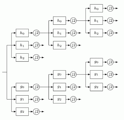
Consequently, the filter bank structure corresponding to the double-density complex DWT consists of two oversampled iterated filter banks operating in parallel on the same input data. (The oversampled filter bank is illustrated in Fig. 1 in this section.) The iterated oversampled filter bank pair, corresponding to the simultaneous implementation of the double-density and dual-tree DWTs, is illustrated in Figure 9 below.

Figure 9.   Iterated Filterbank for the Double-Density Complex DWT.

As you can see, there are two separate filter banks denoted by h_i(n) and g_i(n) where i = 0, 1, 2. The filter banks h_i(n) and g_i(n) are unique and designed in a specific way so the subband signals of the upper DWT can be interpreted as the real part of a complex wavelet transform, and the subband signals of the lower DWT can be interpreted as the imaginary part. Equivalently, for specially designed sets of filters, the wavelets associated with the upper DWT can be approximate Hilbert transforms of the wavelets associated with the lower DWT. When designed in this way, the double-density complex DWT can be used to implement 2-D oriented wavelet transforms, which are especially efficient in image processing. (Recall that for the double-density DWT, four out of the eight wavelets did not have a dominant orientation.) Because of this, the double-density complex DWT is expected to outperform the double-density DWT in various applications, such as image denoising and enhancement. But first we must design the filters for the double-density complex DWT.

The FIR perfect reconstruction filter banks designed for this procedure are displayed below. We implement them by using one set of filter banks for the first stage (FSdoubledualfilt.m) and a second set of filters for the remaining stages (doubledualfilt.m). The filter bank for the remaining stages is designed such that the analysis filters of the first tree are the synthesis filters for the second tree, and vice versa. The function FSdoubledualfilt.m provides analysis and synthesis filter for the first stage of the double-density oriented DWT, while the function doubledualfilt.m provides analysis and synthesis filters for the remaining stages of the transform.

function [af, sf] = FSdoubledualfilt

% USAGE:
%   [af, sf] = FSdoubledualfilt
% OUTPUT:
%   af - cell array containing analysis filters
%       af{1} - analysis filters for tree 1
%       af{2} - analysis fitlers for tree 2
%   sf - cell array containing synthesis filters
%       sf{1} - synthesis filters for tree 1
%       sf{2} - synthesis filters for tree 2

% ANALYSIS FILTERS
af{1} = [
                  0                  0                  0
   0.00069616789827  -0.00014203017443   0.00014203017443
  -0.02692519074183   0.00549320005590  -0.00549320005590
  -0.04145457368920   0.01098019299363  -0.00927404236573
   0.19056483888763  -0.13644909765612   0.07046152309968
   0.58422553883167  -0.21696226276259   0.13542356651691
   0.58422553883167   0.33707999754362  -0.64578354990472
   0.19056483888763   0.33707999754362   0.64578354990472
  -0.04145457368920  -0.21696226276259  -0.13542356651691
  -0.02692519074183  -0.13644909765612  -0.07046152309968
   0.00069616789827   0.01098019299363   0.00927404236573
                  0   0.00549320005590   0.00549320005590
                  0  -0.00014203017443  -0.00014203017443
                  0                  0                  0
];

af{2} = [
                  0                  0                  0
                  0                  0                  0
   0.00069616789827  -0.00014203017443   0.00014203017443
  -0.02692519074183   0.00549320005590  -0.00549320005590
  -0.04145457368920   0.01098019299363  -0.00927404236573
   0.19056483888763  -0.13644909765612   0.07046152309968
   0.58422553883167  -0.21696226276259   0.13542356651691
   0.58422553883167   0.33707999754362  -0.64578354990472
   0.19056483888763   0.33707999754362   0.64578354990472
  -0.04145457368920  -0.21696226276259  -0.13542356651691
  -0.02692519074183  -0.13644909765612  -0.07046152309968
   0.00069616789827   0.01098019299363   0.00927404236573
                  0   0.00549320005590   0.00549320005590
                  0  -0.00014203017443  -0.00014203017443
];

% SYNTHESIS FILTERS
sf{1} = af{1}(end:-1:1, :);
sf{2} = af{2}(end:-1:1, :);

function [af, sf] = doubledualfilt

%% USAGE:
%   [af, sf] = doubledualfilt
% OUTPUT:
%   af - cell array containing analysis filters
%       af{1} - analysis filters for tree 1
%       af{2} - analysis filters for tree 2
%   sf - cell array containing synthesis filters
%       sf{1} - synthesis filters for tree 1
%       sf{2} - synthesis filters for tree 2

% ANALYSIS FILTERS
af{1} = [
   0.00017870679071  -0.00012344587034   0.00001437252392
  -0.02488304194507   0.01718853971559  -0.00200122286479
   0.00737700819766  -0.00675291099550   0.00027261232228
   0.29533805776119   0.02671809818132   0.06840460220387
   0.59529279993637  -0.64763513288874   0.01936710587994
   0.45630440337458   0.47089724990858  -0.68031992557818
   0.11239376309619   0.16040017815754   0.42976785708978
  -0.01971220693439  -0.01484700537727   0.11428688385011
  -0.00813549683439  -0.00588868840296   0.05057805218407
   0.00005956893024   0.00004311757177  -0.00037033761102
];

af{2} = [
   0.00005956893024   0.00004311757177  -0.00037033761102
  -0.00813549683439  -0.00588868840296   0.05057805218407
  -0.01971220693439  -0.01484700537727   0.11428688385011
   0.11239376309619   0.16040017815754   0.42976785708978
   0.45630440337458   0.47089724990858  -0.68031992557818
   0.59529279993637  -0.64763513288874   0.01936710587994
   0.29533805776119   0.02671809818132   0.06840460220387
   0.00737700819766  -0.00675291099550   0.00027261232228
  -0.02488304194507   0.01718853971559  -0.00200122286479
   0.00017870679071  -0.00012344587034   0.00001437252392
];

% Swap the two highpass filters for af{2}
tmp = af{2}(:,2);
af{2}(:,2) = af{2}(:,3);
af{2}(:,3) = tmp;

% SYNTHESIS FILTERS
sf{1} = af{1}(end:-1:1, :);
sf{2} = af{2}(end:-1:1, :);

Summary of Programs

1. FSdoubledualfilt.m - Set of perfect reconstruction filters for the first stage
2. doubledualfilt.m - Set of perfect reconstruction filters for the remaining stages
3. afb3.m - Analysis filter bank
4. sfb3.m - Synthesis filter bank
5. cshift.m - Circular shift