To implement the double-density DWT, we must first select an appropriate filter bank structure. The filter bank proposed in Figure 1 illustrates the basic design of the double-density DWT.
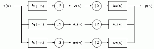
The analysis filter bank consists of three analysis filters—one lowpass filter denoted by h0(-n) and two distinct highpass filters denoted by h1(-n) and h2(-n). As the input signal x(n) travels through the system, the analysis filter bank decomposes it into three subbands, each of which is then down-sampled by 2. From this process we obtain the signals c(n), d1(n), and d2(n), which represent the low frequency (or coarse) subband, and the two high frequency (or detail) subbands, respectively.
The MATLAB program, afb3.m, implements the analysis filter bank. This program utilizes the upfirdn function (found in the Signal Processing Toolbox) to execute the up-sampling, apply a specified FIR filter, and down-sample an input signal x(n).
Matlab Function - afb3.m
function [lo, hi] = afb3(x, af)

%  Analysis Filter Bank
% (consisting of three filters)
%
% USAGE:
%    [lo, hi] = afb3(x, af)
% INPUT:
%     x - N-point vector, where
%            1) N is even
%            2) N >= length(af)
%    af - analysis filters
%    af(:, 1) - lowpass filter (even length)
%    af(:, 2) - first highpass filter (even length)
%    af(:, 3) - second highpass filter (even length)
% OUTPUT:
%     lo - low frequency output
%     hi - cell array containing high frequency outputs
%       1) hi{1} - first high frequency output
%       2) hi{2} - second high frequency output

N = length(x);
L = length(af)/2;
x = cshift(x,-L);

% lowpass filter
lo = upfirdn(x, af(:,1), 1, 2);
lo(1:L) = lo(N/2+[1:L]) + lo(1:L);
lo = lo(1:N/2);

% first highpass filter
hi{1} = upfirdn(x, af(:,2), 1, 2);
hi{1}(1:L) = hi{1}(N/2+[1:L]) + hi{1}(1:L);
hi{1} = hi{1}(1:N/2);

% second highpass filter
hi{2} = upfirdn(x,af(:,3), 1, 2);
hi{2}(1:L) = hi{2}(N/2+[1:L]) + hi{2}(1:L);
hi{2} = hi{2}(1:N/2);
The synthesis filter bank consists of three synthesis filters—one lowpass filter denoted by h0(n) and two distinct highpass filters denoted by h1(n) and h2(n)—which are essentially the inverse of the analysis filters. As the three subband signals travel through the system, they are up-sampled by two, filtered, and then combined to form the output signal y(n). The MATLAB program, sfb3.m, implements the synthesis filter bank.
Matlab Function - sfb3.m
function y = sfb3(lo, hi, sf)

%  Synthesis Filter Bank
% (consisting of three filters)
%
% USAGE:
%    y = sfb3(lo, hi, sf)
% INPUT:
%     lo - low frequency input
%     hi - cell array containing high frequency inputs
%       1) hi{1} - first high frequency input
%       2) hi{2} - second high frequency input
%     sf - synthesis filters
%    sf(:, 1) - lowpass filter (even length)
%    sf(:, 2) - first highpass filter (even length)
%    sf(:, 3) - second highpass filter (even length)
% OUTPUT:
%    y - output signal

N = 2*length(lo);
L = length(sf);
lo  = upfirdn(lo, sf(:,1), 2, 1);
hi{1} = upfirdn(hi{1}, sf(:,2), 2, 1);
hi{2} = upfirdn(hi{2}, sf(:,3), 2, 1);
y = lo + hi{1} + hi{2};
y(1:L-2) = y(1:L-2) + y(N+[1:L-2]);
y = y(1:N);
y = cshift(y, 1-L/2);
One of the main concerns in filter bank design is to ensure the perfect reconstruction (PR) condition. That is, to design h0(n), h1(n), and h2(n) such that y(n)=x(n). To do this, we tested two sets of oversampled filters for the perfect reconstruction condition. The first set of filters (filters1.m) is asymmetric, while the second set of filters (filters2.m) is approximately symmetric. These sets of filters are shown in Tables 1 and 2, respectively.
      h0(-n)            h1(-n)             h2(-n)
 0.14301535070442  -0.01850334430500  -0.04603639605741
 0.51743439976158  -0.06694572860103  -0.16656124565526
 0.63958409200212  -0.07389654873135   0.00312998080994
 0.24429938448107   0.00042268944277   0.67756935957555
-0.07549266151999   0.58114390323763  -0.46810169867282
-0.05462700305610  -0.42222097104302                  0
      h0(-n)	        h1(-n)	            h2(-n)
 0.00069616789827  -0.00014203017443   0.00014203017443
-0.02692519074183   0.00549320005590  -0.00549320005590
-0.04145457368920   0.01098019299363  -0.00927404236573
 0.19056483888763  -0.13644909765612   0.07046152309968
 0.58422553883167  -0.21696226276259   0.13542356651691
 0.58422553883167   0.33707999754362  -0.64578354990472
 0.19056483888763   0.33707999754362   0.64578354990472
-0.04145457368920  -0.21696226276259  -0.13542356651691
-0.02692519074183  -0.13644909765612  -0.07046152309968
 0.00069616789827   0.01098019299363   0.00927404236573
                0   0.00549320005590   0.00549320005590
                0  -0.00014203017443  -0.00014203017443
To verify the perfect reconstruction condition, we can test each oversampled filter bank with a small segment of MATLAB code as shown below. If this condition is satisfied, we know the filter bank will be suitable for use in a double-density DWT application.
EXAMPLE (VERIFY PERFECT RECONSTRUCTION)
>> [af, sf] = filters1;		% analysis and synthesis filters
>> x = rand(1,64);		% create generic signal
>> [lo, hi] = afb3(x, af);	% analysis filter bank
>> y = sfb3(lo, hi, sf);	% synthesis filter bank
>> err = x - y;			% compute error signal
>> max(abs(err))		% verify that error is zero

ans =

  7.6605e-015

>> [af, sf] = filters2;		% analysis and synthesis filters
>> x = rand(1,64);		% create generic signal
>> [lo, hi] = afb3(x, af);	% analysis filter bank
>> y = sfb3(lo, hi, sf);	% synthesis filter bank
>> err = x - y;			% compute error signal
>> max(abs(err))		% verify that error is zero

ans =

  2.6890e-013
After inputting the desired filter, we create a random 1-D signal x of length 64 (or any arbitrary factor of 2). The subband signals (stored in MATLAB as lo, hi{1}, and hi{2}) are then calculated from the analysis filter bank program (afb3.m). We then construct the output signal y using the synthesis filter bank program (sfb3.m). To ensure that the perfect reconstruction condition has been met, we then find the difference between the input signal x and the output signal y. As you can see, the differences found here are significantly close to zero, so much so that they can actually be considered as zero.
Summary of Programs:
- filters1.m - First asymmetric set of perfect reconstruction filters
- filters2.m - Second symmetric set of perfect reconstruction filters
- afb3.m - Analysis filter bank
- sfb3.m - Synthesis filter bank
- cshift.m - Circular shift
Download all framelet programs here. |