Example: Deconvolution using BPD
Deconvolution of a spike signal using basis pursuit denoising.
Ivan Selesnick
NYU-Poly
selesi@poly.edu
March 2012
Contents
Start
close all
clear
MyGraphPrefsON

printme = @(txt) print('-deps', sprintf('figures/Example_deconv_%s',txt));

randn('state',0);           % set state so as to exactly reproduce example
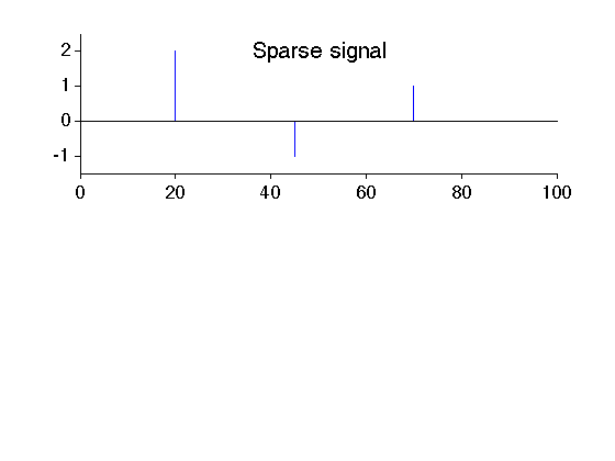
Create spike signal
N = 100;                    % N : length of signal
s = zeros(N,1);
k = [20 45 70];
a = [2 -1 1];
s(k) = a;

figure(1)
clf
subplot(2,1,1)
stem(s, 'marker', 'none')
box off
mytitle('Sparse signal');
ylim1 = [-1.5 2.5];
ylim(ylim1)
xlabel(' ')
printme('original')
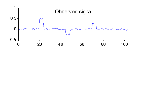
Create observed signal
The simulated observed signal is obtained by convolving the signal with a 4-point impulse response and adding noise.
L = 4;
h = ones(L,1)/L;           % h : impulse response

M = N + L - 1;
w = 0.03 * randn(M,1);     % w : zero-mean Gaussian noise
y = conv(h,s) + w;         % y : observed data

figure(2)
clf
subplot(2,1,1)
plot(y)
box off
xlim([0 M])
mytitle('Observed signal');
xlabel(' ')
printme('observed')
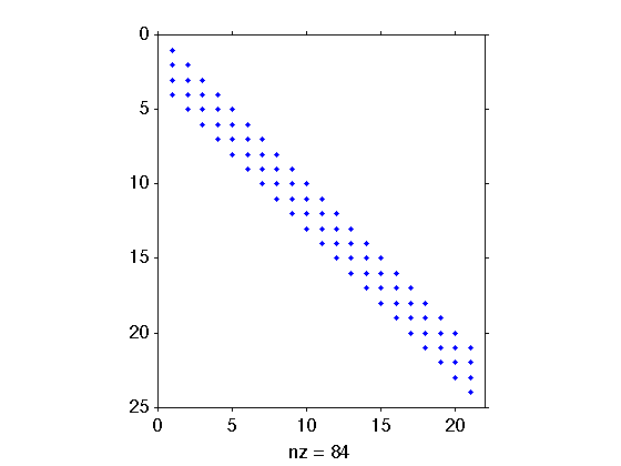
Create convolution matrix H
Create the convolution matrix using Matlab sparse matrix functions 'sparse' and 'spdiags'. By making it a sparse matrix, H uses less memory; multiplying vectors by H will is also faster.
H = sparse(M,N);
e = ones(N,1);
for i = 0:L-1
    H = H + spdiags(h(i+1)*e, -i, M, N);            % H : convolution matrix (sparse)
end
issparse(H)                                         % confirm that H is a sparse matrix
ans =

     1
Verify that H*s is the same as conv(h,s)
err = H*s - conv(h,s);
max_err = max(abs(err));
fprintf('Maximum error = %g\n', max_err)
Maximum error = 0
Display structure of convolution matrix. Note that the matrix is banded (sparse).
figure(1)
clf
spy(H(1:24,1:21))
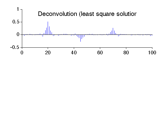
Least square solution
Find the least square solution to the deconvolution problem.
lambda = 0.4;                                       % lambda : regularization parameter

x_L2 = (H'*H + lambda*speye(N)) \ (H' * y);         % x_L2 : least square solution

figure(2)
clf
subplot(2,1,1)
stem(x_L2, 'marker', 'none')
box off
mytitle('Deconvolution (least square solution)');
xlabel(' ')
printme('L2')
Basis pursuit denoising (BPD) solution
Find the BPD solution to the deconvolution problem
% Define algorithm parameters
lambda = 0.05;                                      % lambda : regularization parameter
Nit = 50;                                           % Nit : number of iterations
mu = 0.2;                                           % mu : ADMM parameter

% Run BPD algorithm
[x_BPD, cost] = bpd_salsa_sparsemtx(y, H, lambda, mu, Nit);
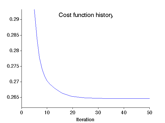
Display cost function history of BPD algorithms
figure(1)
clf
plot(cost)
mytitle('Cost function history');
xlabel('Iteration')
it1 = 5;
del = cost(it1) - min(cost);
ylim([min(cost)-0.1*del cost(it1)])
xlim([0 Nit])
box off
printme('CostFunction')
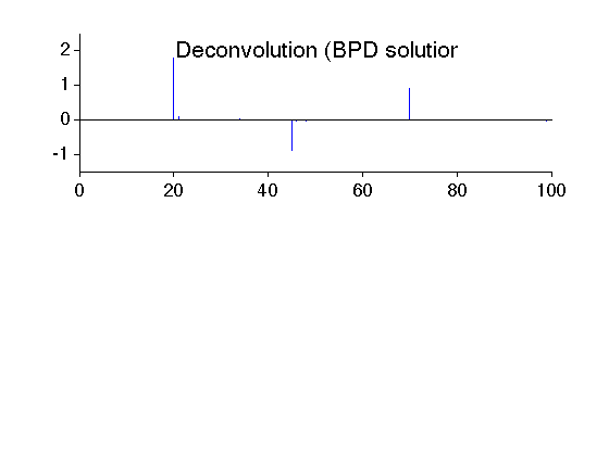
The BPD solution is quite similar to the original signal (much more so than the least square solution).
figure(2)
clf
subplot(2,1,1)
stem(x_BPD, 'marker', 'none')
box off
ylim(ylim1);
mytitle('Deconvolution (BPD solution)');
xlabel(' ')
printme('BPD')
MyGraphPrefsOFF