Example 1: Sparsity-Assisted Signal Smoothing (K = 2)
This example shows the use of SASS for filtering a signal that has discontinuities in its derivative (the signal has cusps). SASS is based on modeling the data, y, as: y = f + g + w where f is a low-pass signal, g has a sparse order-k derivative, and w is white noise.
Ivan Selesnick
selesi@poly.edu
2013
Contents
Start
clear

printme = @(filename) print('-dpdf', sprintf('figures/Example1_%s', filename));

ramp = @(n) n .* (n >= 0);
Make signals
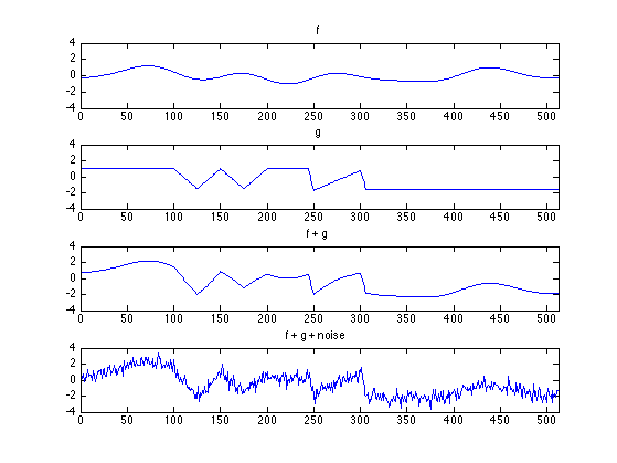
N = 512;
n = (0:N-1)';

% M- : discontinuity points
M1 = 100;
M2 = 125;
M3 = 150;
M4 = 250;
M5 = 250;
M6 = 300;
M7 = 150;
M8 = 175;
M9 = 200;

% g : piecewise linear signal
g = 2 * ramp( n - M1 ) - 4 * ramp( n - M2 ) + 2 * ramp( n - M3 );
g = g + 9 * (ramp(n - M4 + 6) - ramp( n - M4 ));
g = g - ramp( n - M5 ) + 9 * ramp( n - M6 ) - 8 * ramp( n - M6 - 6 );
g = g + 2 * ramp( n - M7 ) - 4 * ramp( n - M8 ) + 2*ramp( n - M9 ) ;
g = 1 - 0.05 * g;

randn('state', 1);
rand('state', 1);               % set rand/randn states for reproducibility of example

f = zeros(size(n));             % f : low-frequency sinusoids
for k = 1:6
    f = f + 0.5 * randn * cos(2*pi*k/N*n + 2*pi*rand);
end

sigma = 0.5;
noise = sigma * randn(size(n)); % noise : white Gaussian noise

s = g + f;                      % s : noise-free signal

data = g + f + noise;           % data : noisy signal
Display signals
ax = [0 N -4 4];

figure(1)
clf

subplot(4, 1, 1)
plot(n, f)
title('f')
axis(ax)

subplot(4, 1, 2)
plot(n, g);
title('g')
axis(ax)

subplot(4, 1, 3)
plot(n, s)
title('f + g')
axis(ax)

subplot(4, 1, 4)
plot(n, data)
title('f + g + noise')
axis(ax)

orient tall
printme('data')
Perform preprocessing
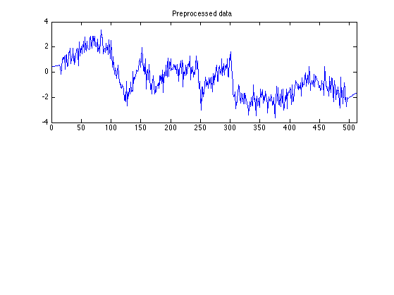
The SASS algorithm may introduce transients at the beginning and end of the signal. To reduce the transients, replace first and last samples of the data by a low-order polynomial approximation.
r = 1;
M = 15;
y = preproc(r, M, data);        % y : preprocessed data

figure(1)
clf
subplot(2, 1, 1)
plot(n, y)
title('Preprocessed data')
xlim([0 N])
Filter matrices
Define filter matrices for SASS.
d = 1;                          % filter is of order 2d
fc = 0.02;                      % fc : cut-off frequency (0 < fc < 0.5) (cycles/sample)
K = 2;                          % K : order of sparse derivative

% Banded filter matrices:
[A, B, B1, D, a, b, b1, H1norm HTH1norm] = ABfilt(d, fc, N, K);
% [A, B] = ABfilt(d, fc, N, K);

H = @(x) [nan(d,1); A\(B*x); nan(d,1)];     % H: high-pass filter
L = @(x) x - H(x);                          % L: low-pass filter

txt_filt = sprintf('d = %d, fc = %.3f', d, fc);
Low-pass filter
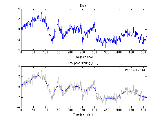
The low-pass filter preserves the low-pass signal, f, with high accuracy, but significantly distorts the piecewise linear signal, g. This guides how to set the cuf-off frequency, fc. fc should be chosen so that the low-pass filter passes the low-pass signal.
x_lpf = L(y);

txt_LPF = sprintf('Low-pass filtering (%s)', txt_filt);

err = s - x_lpf;
RMSE_LPF = sqrt(mean(err(K+1:end-K).^2))

figure(1)
clf

GRAY = [1 1 1]*0.7;

subplot(2, 1, 1)
plot(n, data)
title('Data')
xlabel('Time (samples)')
axis(ax)

subplot(2, 1, 2)
plot(n, data, 'color', GRAY)
line(n, x_lpf);
title('Low-pass filtering (LPF)')
axis(ax)
xlabel('Time (samples)')
axnote(sprintf('RMSE = %.4f', RMSE_LPF))

orient portrait
printme('LPF')
RMSE_LPF =

    0.2513
SASS (L1 norm)
beta = 3;
lam = beta * sigma * HTH1norm;      % lam : regularization parameter

Nit = 100;                          % Nit : number of iterations

[x_L1, cost_L1, u_L1, v_L1] = sass(y, d, fc, K, lam, 'L1', [], Nit);
% x : denoised signal
% cost : cost function history
% u : sparse order-K derivative
% v : inv(A)*B1*u

txt_L1 = sprintf('SASS (L1, K = %d, \\lambda = %.2f, %s)', K, lam, txt_filt)

err = s - x_L1;
RMSE_L1 = sqrt(mean(err(K+1:end-K).^2))
0 incorrectly locked zeros detected.

txt_L1 =

SASS (L1, K = 2, \lambda = 6.00, d = 1, fc = 0.020)


RMSE_L1 =

    0.1430
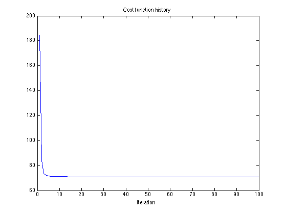
Cost function
figure(2)
clf
plot(cost_L1)
title('Cost function history');
xlabel('Iteration')
Denoised signal
figure(2)
clf
subplot(2, 1, 1)
plot(n, x_L1)
axnote(sprintf('RMSE = %.4f', RMSE_L1))
title(txt_L1)
axis(ax)

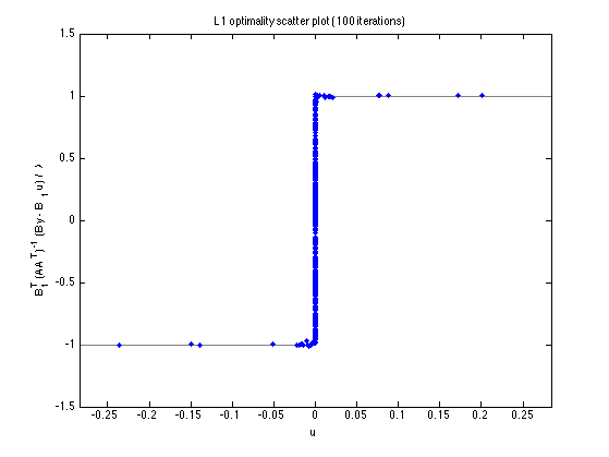
Optimality scatter plot
figure(2)
clf
plot_scatter(A, B, B1, y, u_L1, lam, 'L1', []);
title(sprintf('L1 optimality scatter plot (%d iterations)', Nit))
printme('L1_scatter')
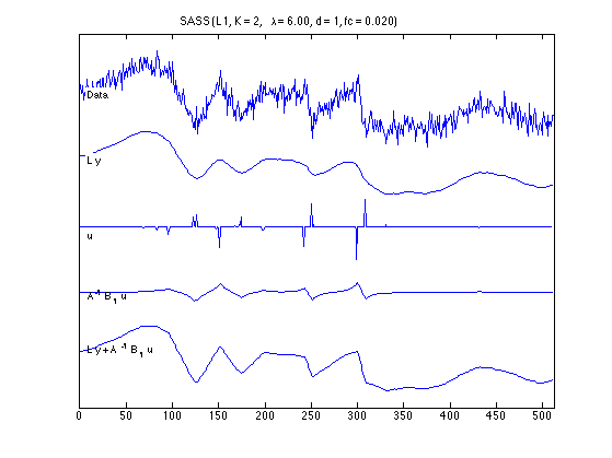
Components
figure(1)
clf
plot_components(n, data, x_lpf, x_L1, u_L1, v_L1, txt_L1);
orient tall
printme('L1_components')
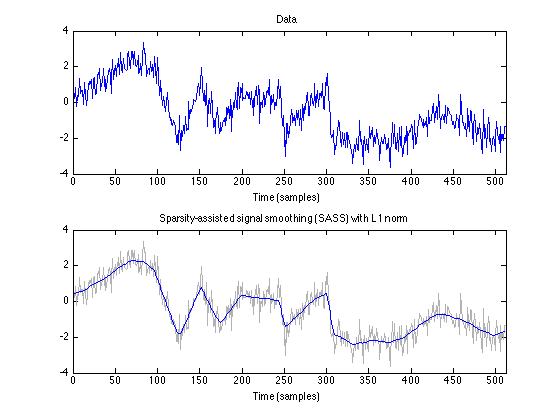
figure(1)
clf

subplot(2, 1, 1)
plot(n, data)
title('Data')
xlabel('Time (samples)')
axis(ax)

subplot(2, 1, 2)
plot( n, data, 'color', GRAY);
line( n, x_L1 );
title('Sparsity-assisted signal smoothing (SASS) with L1 norm')
xlabel('Time (samples)')
axis(ax)

orient portrait
printme('L1')
SASS (log penalty)
The log penalty function is non-convex
% rho : Controls non-convexity of penalty (0 <= rho <= 1)
rho = 0.5;

% initialize with L1 solution
[x_log, cost_log, u_log, v_log, a] = sass(y, d, fc, K, lam, 'log', rho, Nit, u_L1);

txt_log = sprintf('SASS (log, K = %d, \\lambda = %.2f, \\rho = %.2f, %s)', K, lam, rho, txt_filt);

err = s - x_log;
RMSE_log = sqrt(mean(err(K+1:end-K).^2))
0 incorrectly locked zeros detected.

RMSE_log =

    0.1278
Cost function
figure(2)
clf
plot(cost_L1)
title('Cost function history');
xlabel('Iteration')

Denoised signal
figure(2)
clf
subplot(2, 1, 1)
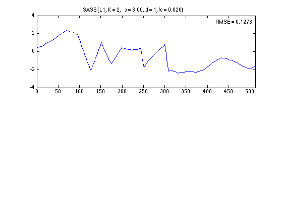
plot(n, x_log)
title(txt_L1)
axnote(sprintf('RMSE = %.4f', RMSE_log))
axis(ax)
Optimality scatter plot
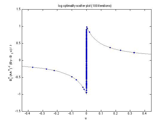
figure(2)
clf
plot_scatter(A, B, B1, y, u_log, lam, 'log', a);
title(sprintf('log optimality scatter plot (%d iterations)', Nit))
printme('log_satter')
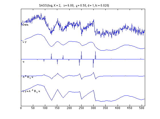
Components
figure(1)
clf
plot_components(n, data, x_lpf, x_log, u_log, v_log, txt_log);
orient tall
printme('log_components')
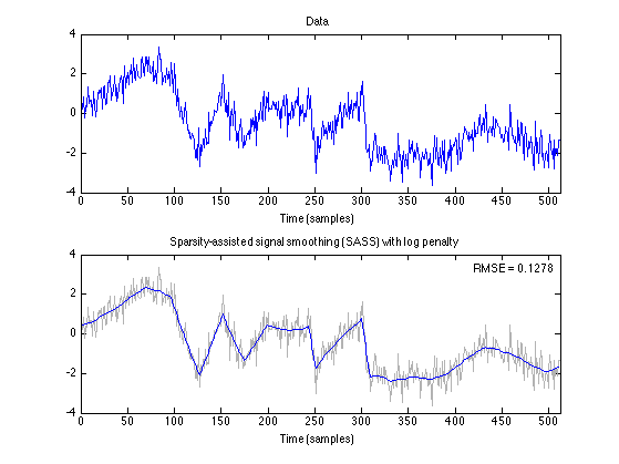
figure(1)
clf

subplot(2, 1, 1)
plot(n, data)
title('Data')
xlabel('Time (samples)')
axis(ax)

subplot(2, 1, 2)
plot( n, data, 'color', GRAY);
line( n, x_log );
title('Sparsity-assisted signal smoothing (SASS) with log penalty')
% title(txt_log)
axnote(sprintf('RMSE = %.4f', RMSE_log))
xlabel('Time (samples)')
axis(ax)

orient portrait
printme('log')
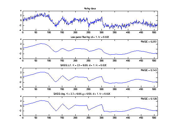
Save figure to pdf file
set(0, 'DefaultAxesFontSize', 8);

figure(10)
clf

M = 4;

subplot(M, 1, 1)
plot(n, data)
title('Noisy data');
axis(ax)

subplot(M, 1, 2)
plot(n, x_lpf);
title(txt_LPF)
axnote(sprintf('RMSE = %.3f', RMSE_LPF))
axis(ax)

subplot(M, 1, 3)
plot(n, x_L1)
title(txt_L1);
axnote(sprintf('RMSE = %.3f', RMSE_L1))
axis(ax)

subplot(M, 1, 4)
plot(n, x_log)
title(txt_log);
axnote(sprintf('RMSE = %.3f', RMSE_log))
axis(ax)

orient tall
printme('fig1')

set(0, 'DefaultAxesFontSize', 'remove');