demo_simulated_ECG: signal denoising using SASS

Ivan Selesnick
selesi@nyu.edu
2013, revised 2016, 2017

Contents

Start

clear

compute_rmse = @(err) sqrt(mean(abs(err(:)).^2));

Load data

% load simulated ECG
s = load('data/simulated_ecg.txt');

% load simulated ECG plus noise
y = load('data/simulated_ecg_noisy.txt');

sigma = 0.2;

N = length(s);
n = 0:N-1;

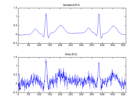
Display ECG signals

ax = [0 N -0.5 1.5];

figure(1)
clf
subplot(2, 1, 1)
plot(n, s)
title('Simulated ECG')
axis(ax)

subplot(2, 1, 2)
plot(n, y)
title('Noisy ECG');
axis(ax)

Parameters

% Filter parameters:
% d  : filter order parameter (the filter is of order 2d)
% fc : cut-off frequency (0 < fc < 0.5) (cycles/sample)

% SASS parameters
% K : order of sparse derivative
% lam : regularization parameter

% Uncomment one of the following lines to select parameter values
% PARAMVALS = 1;
PARAMVALS = 2;

switch PARAMVALS
    case 1
        % low-pass filter parameters
        d = 1;             % 2nd order filter
        fc = 0.03;
        % SASS parameters
        K = 2;
        lam = 1.3;
    case 2
        % low-pass filter parameters
        d = 2;             % 4th order filter
        fc = 0.03;
        % SASS parameters
        K = 2;
        lam = 1.52;
end

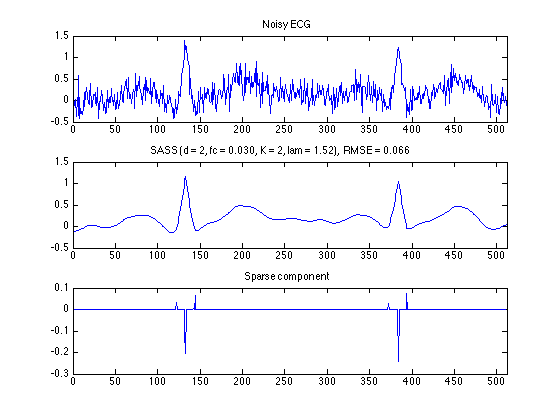
SASS - run algorithm

[x, u] = sass_L1(y, d, fc, K, lam);
% x : denoised signal
% u : sparse order-K derivative

RMSE = compute_rmse(s - x);

0 incorrectly locked zeros detected.

SASS - plot denoised signal

txt = sprintf('SASS (d = %d, fc = %.3f, K = %d, lam = %.2f),  RMSE = %.3f', d, fc, K, lam, RMSE);

figure(1)
clf
subplot(3, 1, 1)
plot(n, y)
title('Noisy ECG');
axis(ax)

subplot(3, 1, 2)
plot(n, x)
title(txt)
axis(ax)

subplot(3, 1, 3)
plot(u)
xlim([0 N])
title('Sparse component')

orient tall
print('-dpdf', sprintf('figures/demo_simulated_ECG_%d', PARAMVALS))

Compare to low-pass filter

[A, B, B1] = ABfilt(d, fc, N, K);   % Filter matrices (banded)

H = @(x) A\(B*x);           % H: high-pass filter
L = @(x) x - H(x);          % L: low-pass filter

x_lpf = L(y);

RMSE_lpf = compute_rmse(s - x_lpf);

txt_lpf = sprintf('Low-pass filter, RMSE = %.3f', RMSE_lpf);

figure(1)
clf
subplot(2, 1, 1)
plot(n, x)
title(txt)
axis(ax)

subplot(2, 1, 2)
plot(n, x_lpf)
title(txt_lpf)
axis(ax)

orient portrait
print('-dpdf', sprintf('figures/demo_simulated_ECG_LPF_%d', PARAMVALS))

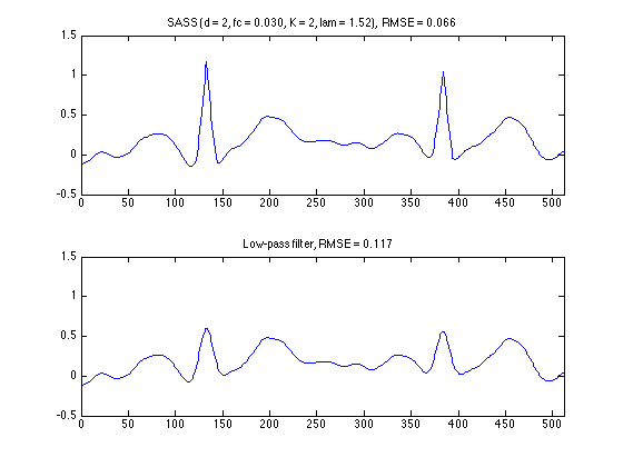
The low-pass filter recovers a low-pass signal (f) but significantly distorts the piecewise linear signal (g). Adjusting the low-pass filter helps to set the cuf-off frequency, fc. The cut-off frequency should be chosen so the low-pass filter preserves the low-frequency content of the signal.

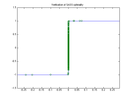
SASS - optimality scatter plot

Verify the solution satisfies the optimality condition

[A, B, B1] = ABfilt(d, fc, N, K);   % Filter matrices (banded)

r = B1' * ((A*A')\(B*y-B1*u)) / lam;
M = 1.2 * max(abs(u));

figure(1)
clf
plot([-M 0 0 M], [-1 -1 1 1], u, r, 'o')
title('Verification of SASS optimality')
axis([-M M -1.5 1.5])

orient portrait
print -dpdf figures/demo_simulated_ECG_optimality_plot

Published with MATLAB® 7.12