Example 3: Filtering biosensor data using the LoPATV algorithm
Filtering of biosensor data using local least-square polynomial approximation and total variation filtering (LoPATV filter)
Ivan Selesnick,
Polytechnic Institute of NYU
December 2011
Email: selesi@poly.edu
Reference: Polynomial Smoothing of Time Series with Additive Step Discontinuities
I. W. Selesnick, S. Arnold, and V. R. Dantham
Contents
Start
clear
close all

printme = @(filename) print('-dpdf', sprintf('figures/Example3_%s', filename));
Load data
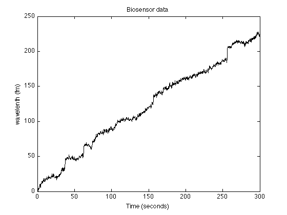
load wgm_data.txt       % load WGM sensor data

y = wgm_data;
N = length(y);          % N : 1500
n = 1:N;
t = (0:N-1)/5;          % t : time axis (sampling rate is 5 samples/second)

figure(1)
clf
plot(t, y, 'black')
title('Biosensor data');
xlabel('Time (seconds)')
ylabel('wavelenth (fm)')
printme('data')
LoPATV filtering
Local polynomial approximation + total variation filter
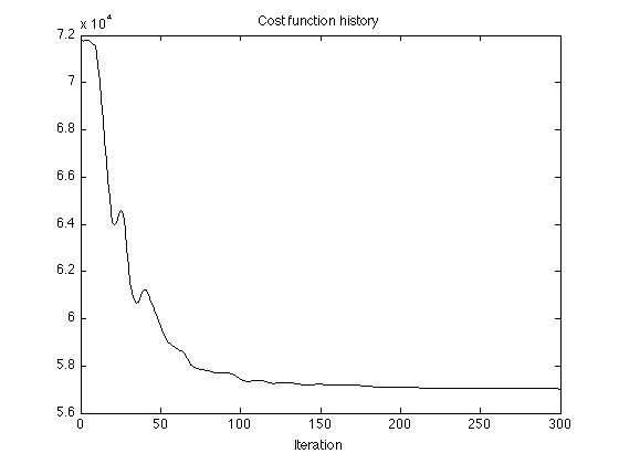
lambda = 600;       % lambda : TV regularization parameter
L = 200;            % L : block length
P = 150;            % P : block overlap
deg = 1;            % deg : degree of polynomial

(N-L)/(L-P)+1       % This is the number of blocks - it should be an
                    % integer, otherwise the data will be truncated

mu0 = 500;
mu = .05;
Nit = 300;

[x, s, cost] = lopatv(y, L, P, deg, lambda, Nit, mu0, mu);
% x : TV component (approximate step signal)
% s : smooth low-pass signal
% cost : cost function history

figure(1)
plot(cost, 'black')
title('Cost function history')
xlabel('Iteration')
ans =

    27
Display filtered data
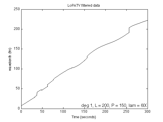
txt = sprintf('deg %d, L = %d, P = %d, lam = %.f', deg, L, P, lambda);

figure(1)
clf
plot(t, x+s, 'black')
xlabel('Time (seconds)')
ylabel('wavelenth (fm)')
title('LoPATV filtered data')
text(0.99, 0.01, txt, 'units', 'normalized', 'horizontalalignment', 'right', 'verticalalignment', 'bottom', 'fontsize', 12);
printme('LoPATV')
Display step signal
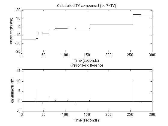
figure(2)
clf
subplot(2,1,1)
plot(t, x, 'black')
title('Calculated TV component (LoPATV)');
ylim([-30 21])
ylabel('wavelength (fm)')
xlabel('Time (seconds)')

subplot(2,1,2)
stem(t(1:end-1), diff(x), 'marker','none', 'color', 'black')
title('First-order difference');
ylim([-5 16])
ylabel('wavelength (fm)')
xlabel('Time (seconds)')

printme('LoPATV_steps')
Enhanced LoPATV filtering
Lp quasi-norm minimization
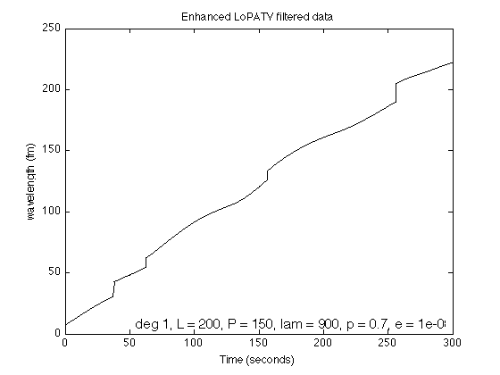
p = 0.7;
E = 1e-8;
lambda = 900;

[x, s, cost] = lopatv_Lp(y, L, P, deg, lambda, Nit, mu0, mu, p, E);

figure(1)
clf
plot(t, s+x, 'black');
xlabel('Time (seconds)')
ylabel('wavelength (fm)')
title('Enhanced LoPATV filtered data')

txt = sprintf('deg %d, L = %d, P = %d, lam = %.f, p = %.1f, e = %.2g', deg, L, P, lambda, p, E);
h = text(0.98, 0.01, txt, 'units', 'normalized', 'horizontalalignment', 'right', 'verticalalignment', 'bottom', 'fontsize', 12);

printme('enhanced_LoPATV')
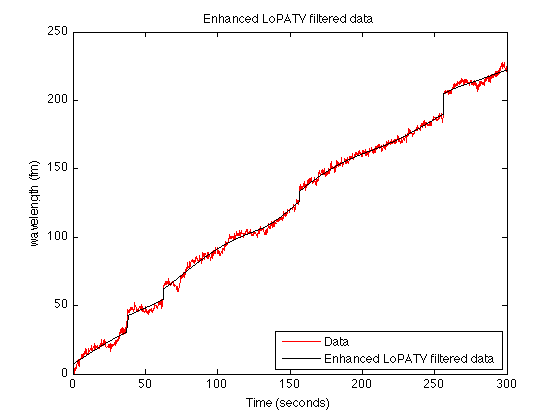
figure(1)
clf
plot(t, y, 'color', 'red');
line(t, x+s,'linewidth',1,'color','black')
legend('Data','Enhanced LoPATV filtered data', 'location','southeast')
xlabel('Time (seconds)')
ylabel('wavelength (fm)')
title('Enhanced LoPATV filtered data')
printme('enhanced_LoPATV_fig2')
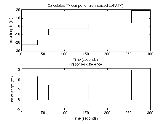
Display step signal
figure(2)
clf
subplot(2,1,1)
plot(t, x, 'black')
title('x(t)');
ylim([-30 21])
ylabel('wavelength (fm)')
xlabel('Time (seconds)')
title('Calculated TV component (enhanced LoPATV)');

subplot(2,1,2)
stem(t(1:end-1), diff(x),'marker','none', 'color', 'black')
title('First-order difference');
xlabel('Time (seconds)')
ylim([-5 16])
ylabel('wavelength (fm)')

printme('enhanced_LoPATV_steps')