Example 1: Polynomial approximation + total variation filtering
Example: Simultaneous least-square polynomial approximation and total variation filtering. The algorithm in derived using majorization-minimization (MM).
Ivan Selesnick,
Polytechnic Institute of NYU
Contents
Start
clear
close all
% addpath extra_functions/

printme = @(filename) print('-dpdf', sprintf('figures/Example1_%s', filename));
Create test signals
N = 100;                            % N : length of data
n = (1:N)';
s1 = n < 0.3*N;                     % s1 : step function
s2 = 2-2*((n-N/2)/(N/2)).^2;
s2 = s2 + n/N;                      % s2 : polynomial function

randn('state',0);                   % Initialize randn so that example can be exactly reproduced
sigma = 0.25;
noise = sigma * randn(N,1);
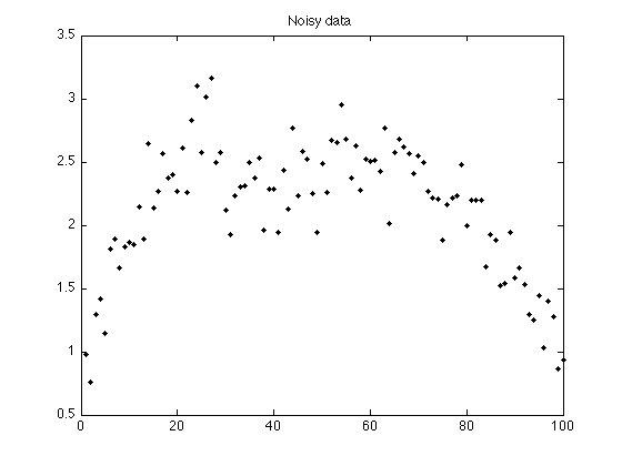
Create noisy signal
Create polynomial signal with additive step discontinuity
s = s1 + s2;                % s : polynomial signal with additive step discontinuity
y = s + noise;              % y : noisy signal

figure(1)
plot(n, y, '.k')
title('Noisy data');
printme('data')
Perform PATV filtering
PATV: Least square polynomial approximation + total variation denoising
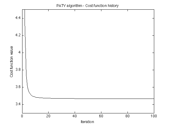
% parameters
d = 2;                          % d : degree of approximation polynomial
lam = 1.5;                      % lambda : regularization parameter
Nit = 100;                      % Nit : number of iterations

[x, p, cost, u, v] = patv_MM(y, d, lam, Nit);

% display cost function history
figure(1)
plot(1:Nit, cost)
title('PATV algorithm - Cost function history');
xlabel('Iteration')
ylabel('Cost function value')
ylim([3.3 4.5])
printme('convergence')
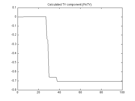
Display calculated TV component
figure(1)
clf
plot(n, x, 'k')
title('Calculated TV component (PATV)');
printme('TV_component')
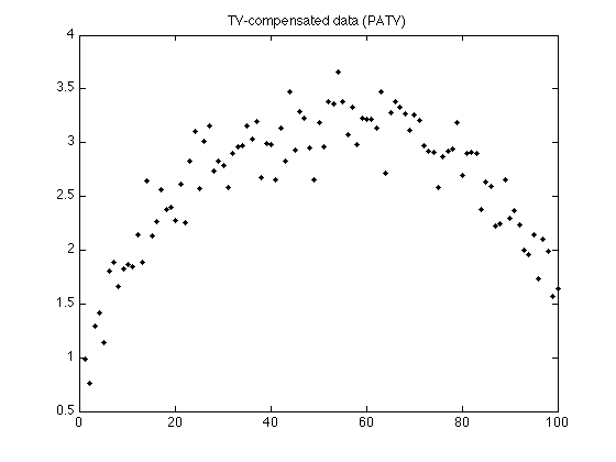
Display TV-compensated data
figure(2)
clf
plot(n, y - x, '.k')
title('TV-compensated data (PATV)');
printme('TV_compensated_data')
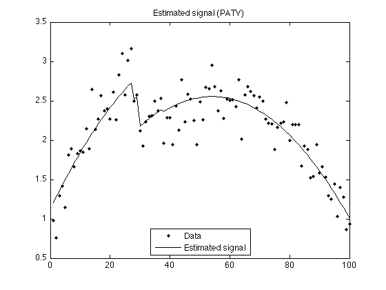
Display estimated signal
figure(1)
clf
plot(n, y,'.k', n, x+p, 'black')
title('Estimated signal (PATV)');
legend('Data','Estimated signal', 'Location','south')
printme('PATV')
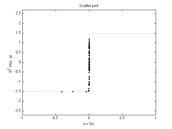
Optimality scatter plot
phi_L1 = @(x) lam * abs(x);
wfun_L1 = @(x) abs(x)/lam;
dphi_L1 = @(x) lam * sign(x);

t = [linspace(-1, -eps, 100) linspace(eps, 1, 100)];

MS = 8;

figure(1)
plot( u, v, '.' , 'markersize', MS)
line(t, dphi_L1(t), 'linestyle', ':')
ylim([-1 1] * lam * 1.8)
xlabel('u = Dx')
ylabel('S^T H(y - x)')
title('Scatter plot');
printme('scatter')
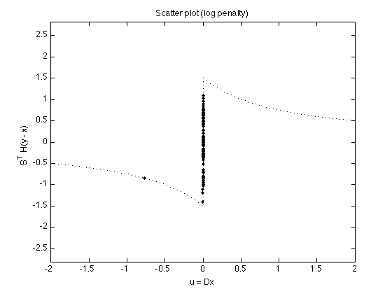
PATV with logarithmic penalty
lam = 1.5;
a = 1.0;
% a = eps;    % L1 norm - reproduces above result

phi = @(x) lam/a * log(1 + a*abs(x));
dphi = @(x) lam ./(1 + a*abs(x)) .* sign(x);
wfun = @(x) abs(x) .* (1 + a*abs(x)) / lam;

[x2, p2, cost2, u, v] = patv_MM2(y, d, phi, wfun, Nit);

t = [linspace(-2, -eps, 100) linspace(eps, 2, 100)];

figure(1)
plot( u, v, '.' , 'markersize', MS)
line(t, dphi(t), 'linestyle', ':')
ylim([-1 1] * max(abs(v)) * 2)
xlabel('u = Dx')
ylabel('S^T H(y - x)')
title('Scatter plot (log penalty)');
printme('scatter_log')
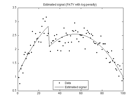
Display estimated signal
figure(2)
clf
plot(n, y,'.k', n, x2+p2, 'black')
title('Estimated signal (PATV with log penalty)');
legend('Data','Estimated signal', 'Location','south')
printme('PATV_log')