demo3: group-sparse thresholding, 3D data
This example illustrates 3D sparse signal denoising using non-convex overlapping group sparsity (OGS).
This demo illustrates the non-convex form of OGS, with two different non-convex penalties: atan and MCP.
Ivan Selesnick, July 2014. Revised, May 2016.
Reference: P. Y. Chen and I. W. Selesnick, "Group-Sparse Signal Denoising: Non-Convex Regularization, Convex Optimization," IEEE Transactions on Signal Processing, vol. 62, no. 13, pp. 3464-3478, July 1, 2014. doi: 10.1109/TSP.2014.2329274
Contents
Set up
clear
close all

% Set random number generator for reproducibility
rng('default')
rng(1)

rmse = @(err) sqrt(mean(abs(err(:)).^2));
Make data
% N : size of 3D data
N = [30, 40, 20];

% s : noise-free data
s = zeros(N);
s(10+(1:4), 10+(1:4), 10+(1:4)) = rand(4,4,4)-0.5;
s(15+(1:4), 25+(1:4), 8+(1:4)) = rand(4,4,4)-0.5;

% y : noisy data
sigma = 0.1;
y = s + sigma * randn(N);
Denoising using OGS
K = [3 3 3];       % K : group size
% Note: the group size does not need to be the same as
% the true groups in the data. Usually, the specified
% group size should be smaller. (Also, in many real data,
% groups are of different sizes anyway, there is not
% single group size to identify.)

% OGS (atan penalty (default))
lam = 0.027;
x1 = ogs3(y, K, lam);
rmse(x1 - s)

% OGS (mcp penalty)
pen = 'mcp';
lam = 0.027;
x2 = ogs3(y, K, lam, pen);
rmse(x2 - s)
ans =

          0.01


ans =

          0.01
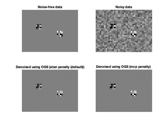
Display 2D slices
Show 2D slices through the data as images
Clim = [-1 1]/2;  % color limits

figure(1)
clf

subplot(2, 2, 1)
imagesc(s(:,:,11), Clim)
title('Noise-free data');
colormap(gray(256))
axis image off

subplot(2, 2, 2)
imagesc(y(:,:,11), Clim)
title('Noisy data');
axis image off

subplot(2, 2, 3)
imagesc(x1(:,:,11), Clim)
title('Denoised using OGS (atan penalty (default))');
axis image off

subplot(2, 2, 4)
imagesc(x2(:,:,11), Clim)
title('Denoised using OGS (mcp penalty) ');
axis image off

orient landscape
print -dpdf -fillpage figures/demo3_fig1
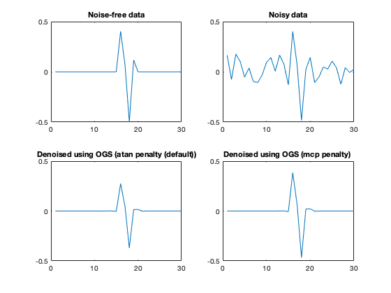
Display 1D lines
Display 1D lines through the data as plots. The 'mcp' penalty does a little better than the default ('atan') penalty. Both are non-convex penalties.
figure(2)
clf

subplot(2, 2, 1)
plot(s(:,26,11))
title('Noise-free data');
ylim(Clim)

subplot(2, 2, 2)
plot(y(:,26,11))
title('Noisy data');
ylim(Clim)

subplot(2, 2, 3)
plot(x1(:,26,11))
title('Denoised using OGS (atan penalty (default))');
ylim(Clim)

subplot(2, 2, 4)
plot(x2(:,26,11))
title('Denoised using OGS (mcp penalty) ');
ylim(Clim)

orient landscape
print -dpdf -fillpage figures/demo3_fig2