LPFTVD_Example_2

Filtering NIRS time-series data with the LPF/TVD algorithm.

The main parameters are:

Ivan Selesnick,
Polytechnic Institute of NYU,
June 2012

Contents

Start

clear
% close all

printme = @(filename) print('-dpdf', sprintf('figures/LPFTVD_Example_2_%s', filename));

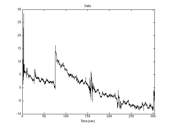
Load data

y = load('wl2_col38.txt');

Fs = 6.25;          % Fs : sampling rate (samples/second)
N = length(y);
n = 1:N;
t = n/Fs;

figure(1)
clf
plot(t, y);
xlim([0 N/Fs])
ax1 = axis;
axis(ax1);
title('Data')
xlabel('Time (sec)')

Set filter parameters

Set filter parameters, fc and d.

fc = 0.02;       % fc : cut-off frequency (cycles/sample) (0 < fc < 0.5);
d = 1;           % d : filter order parameter (d = 1, 2, or 3)

fprintf('LPF cut-off frequency: %f cycles/sec \n', fc * Fs);

LPF cut-off frequency: 0.125000 cycles/sec 

Run LPF/TVD algorithm

lam = 1.2;
% lam : positive regularization parameter

Nit = 30;
% Nit : number of iterations

[x, f, cost] = lpftvd(y, d, fc, lam, Nit);       % Run LPF/TVD algorithm

txt = sprintf('fc = %.2e, d = %d, lam = %.2e', fc, d, lam);

if 0
    % Run-time computation
    tic
    for ii = 1:50
        [x_, f_, cost_] = lpftvd(y, d, fc, lam, Nit);
    end
    run_time = toc/50;
    fprintf('LPF/TVD run-time: %.4f seconds (length = %d samples, %d iterations)\n', run_time, length(y), Nit);
end

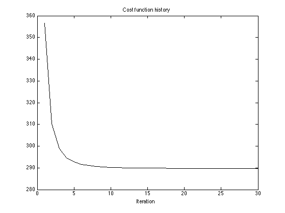
Display cost function history

figure(1)
clf
plot(cost)
title('Cost function history');
xlabel('Iteration')

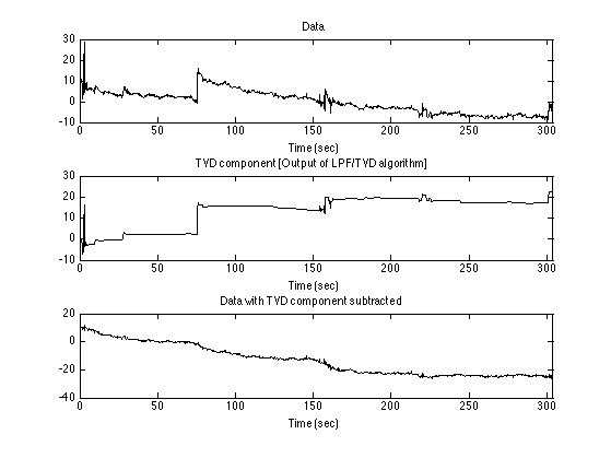
Display output of LPF/TVD

figure(2)
clf

subplot(3, 1, 1)
plot(t, y)
xlim([0 N/Fs])
ax = axis;
title('Data')
axis(ax)
xlabel('Time (sec)')

subplot(3, 1, 2)
plot(t, x)
title('TVD component [Output of LPF/TVD algorithm]')
xlim([0 N/Fs])
xlabel(txt)
axis(ax)
xlabel('Time (sec)')

subplot(3, 1, 3)
plot(t, y - x)
xlim([0 N/Fs])
xlabel('Time (sec)')
title('Data with TVD component subtracted')

orient tall
printme('lpftvd')

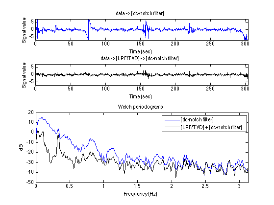
Dc-notch filtering

Apply dc-notch filter for baseline removal. Compute the periodogram after baseline removal. Do the same for data with TVD component subtracted.

y2 = y - x;                 % y2 : data with TVD component subtracted

b = [1 -1];                 % b, a : coefficients of dc-notch filter
a = [1 -0.96];

g = filtfilt(b, a, y);      % apply dc-notch filter to y
g2 = filtfilt(b, a, y2);    % apply dc-notch filter to y2

G = pwelch(g);              % Welch periodograms
G2 = pwelch(g2);

L = length(G2) - 1;
f = (0:L)/L * Fs/2;         % f : frequency axis for periodograms

Display periodograms

Display signals and periodograms with and without LPF/TVD processing to remove TV component.

figure(5)
clf

subplot(4, 1, 1)
plot(t, g, 'b')
xlim([0 N/Fs])
xlim2 = [-7 7];
ylim(xlim2)
title('data -> [dc-notch filter]')
xlabel('Time (sec)')
ylabel('Signal value')

subplot(4, 1, 2)
plot(t, g2, 'k')
ylim(xlim2)
xlim([0 N/Fs])
title('data -> [LPF/TVD] -> [dc-notch filter]')
xlabel('Time (sec)')
ylabel('Signal value')

subplot(2, 1, 2)
plot(f, 20*log10(G), 'b' )
line(f, 20*log10(G2), 'color', 'k' );
xlabel('Frequency (Hz)')
ylim([-50 20])
title('Welch periodograms')
legend('[dc-notch filter]', '[LPF/TVD] + [dc-notch filter]')
ylabel('dB')

xlim([0 Fs/2])

orient tall
printme('welch')

Published with MATLAB® 7.12