Example: Basis pursuit (BP)

In this example, we obtain frequency-domain coefficients of a sinusoid using three methods:

As illustrated in the example, the coefficients obtained using basis pursuit are sparse and do not exhibit the leakage phenomenon.

Ivan Selesnick
NYU-Poly
selesi@poly.edu
March 2012

Contents

Start

close all
clear
I = sqrt(-1);

printme = @(txt) print('-dpdf', sprintf('figures/Example_BP_%s',txt));

function 'A'

The function 'A' maps an N-point coefficient vector c to an M-point signal y (where M <= N).

type A

function y = A(c, M, N)
    v = N * ifft(c);
    y = v(1:M);
end

function 'AT'

The function 'AT' maps an M-point signal y to an N-point coefficient vector c (where M <= N). 'AT' is the complex conjugate transpose of 'A'.

type AT

function c = AT(y, M, N)
    c = fft([y; zeros(N-M, 1)]);
end

Perfect reconstruction

Verify the perfect reconstruction property of A and AT. (Show that A*AT = N*identity)

M = 100;
N = 256;
y = rand(M,1);
c = (1/N)*AT(y, M, N);
y2 = A(c, M, N);
recon_err = y2 - y;   % recon_err : reconstruction error

fprintf('Maximum reconstruction error : %g\n', max(recon_err))

Maximum reconstruction error : 4.44089e-16

Create signal

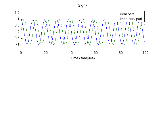
The signal consists of 100 points of a complex sinusoid.

M = 100;
m = (0:M-1)';

f1 = 10.5;
x = exp(I*2*pi*f1/M*m);             % x : signal

figure(1)
clf
subplot(2,1,1)
plot(m, real(x), m, imag(x),'--')
xlabel('Time (samples)')
title('Signal');
legend('Real part','Imaginary part')
box off
ylim1 = [-1.4 1.8];
ylim(ylim1)
printme('signal')

Spectrum (using DFT)

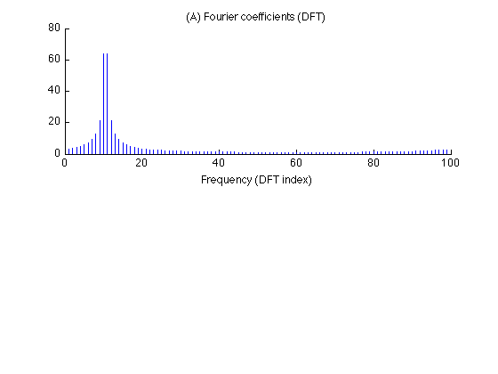
Compute the DFT of the signal. Note that the spectrum (DFT) of the signal exhibits leakage. This is because the signal consists of 10.5 cycles of a sinusoid (not a whole number of cycles).

X = fft(x);                         % X : DFT of x

subplot(2,1,1)
stem(m,abs(X),'marker','none')
xlabel('Frequency (DFT index)')
title('(A) Fourier coefficients (DFT)');
box off
printme('DFT')

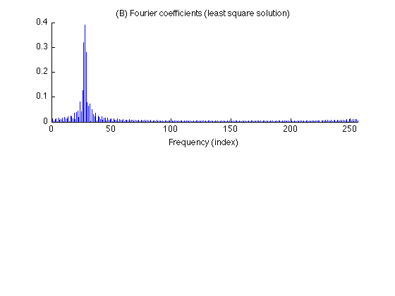
Oversampled DFT: Least squares

Compute the oversampled DFT of the signal using function 'AT'. Note that the obtained spectrum exhibits leakage again. Because the oversampled DFT is a Parseval frame, the least square solution is obtained by the conjugate transpose (and normalization by N).

N = 256;
X = (1/N)*AT(x,M,N);

figure(2)
clf
subplot(2,1,1)
stem(abs(X),'marker','none')
title('(B) Fourier coefficients (least square solution)');
xlabel('Frequency (index)')
box off
xlim([0 N])
printme('LeastSquares')

Verify reconstruction of least square solution

err = x - A(X,M,N);
err_max = max(abs(err));
fprintf('Least squares: Maximum reconstruction error = %g\n', err_max);

Least squares: Maximum reconstruction error = 5.55805e-16

Oversampled DFT: Basis pursuit

% Define functions (Matlab function handles)
H = @(x) A(x,M,N);
HT = @(x) AT(x,M,N);

% Define algorithm parameters
p = N;                  % p : Parseval constant
Nit = 100;              % Nit : number of iterations
mu = 5;                 % mu : ADMM parameter

% Run basis pursuit algorithm
[c, cost] = bp_salsa(x, H, HT, p, mu, Nit);

Verify reconstruction of basis pursuit solution

err = x - A(c,M,N);
err_max = max(abs(err));
fprintf('Basis pursuit: Maximum reconstruction error = %g\n', err_max);

Basis pursuit: Maximum reconstruction error = 1.26585e-15

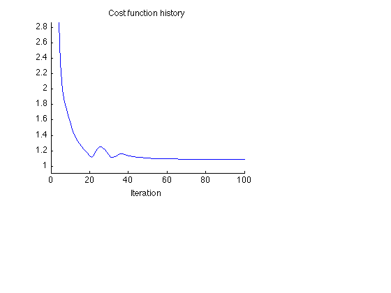
Display cost function history of basis pursuit algorithm

figure(1)
clf
subplot(3,3,[1 2 4 5])
plot(cost)
title('Cost function history');
xlabel('Iteration')
it1 = 4;
del = cost(it1) - min(cost);
ylim([min(cost)-0.1*del cost(it1)])
xlim([0 Nit])
box off
printme('CostFunction')

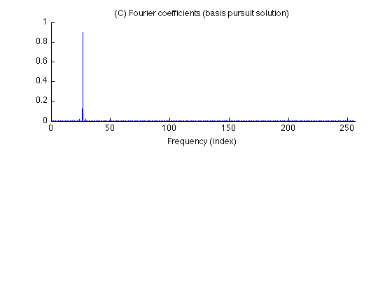
Display Fourier coefficients obtained by basis pursuit

figure(2)
clf
subplot(2,1,1)
stem(0:N-1, abs(c), 'marker','none')
title('(C) Fourier coefficients (basis pursuit solution)');
xlabel('Frequency (index)')
box off
xlim([0 N])
printme('BasisPursuit')

Published with MATLAB® 7.8