Least square polynomial approximation
This example illustrates the fitting of a low-order polynomial to data by least squares.
Ivan Selesnick
selesi@poly.edu
Contents
Start
clear
close all
Load data
load data.txt;
whos

t = data(:, 1);         % time index
y = data(:, 2);         % data value
  Name        Size            Bytes  Class     Attributes

  data      100x2              1600  double
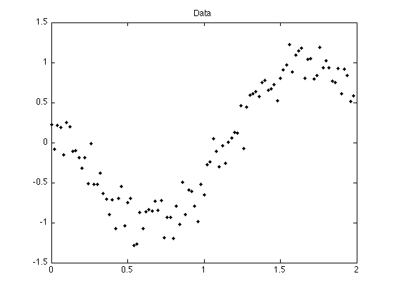
Display data
figure(1)
clf
plot(t, y, '.')
title('Data')
Polynomial approximation (degree = 2)
A is a matrix of size 100 rows, 3 columns
A = bsxfun(@power, t, [2 1 0]);       % Raise t to powers 2, 1, 0
size(A)
ans =

   100     3
A'*A is a matrix of size 3 by 3
A'*A
ans =

  312.0533  196.0200  131.3400
  196.0200  131.3400   99.0000
  131.3400   99.0000  100.0000
Solve the system A'*A*p = A'*y for p using the backslash. p is a vector of length 3.
p = (A'*A) \ (A'*y)
p =

    1.0620
   -1.1989
   -0.2236
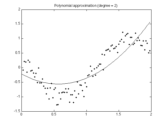
Display polynomial approximation
plot(t, polyval(p, t), t, y, '.')
title('Polynomial approximation (degree = 2)')
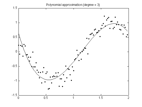
Polynomial approximation (degree = 3)
A = bsxfun(@power, t, [3 2 1 0]);
p = (A'*A) \ (A'*y);

plot(t, polyval(p, t), t, y, '.')
title('Polynomial approximation (degree = 3)')
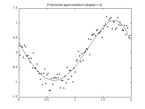
Polynomial approximation (degree = 4)
A = bsxfun(@power, t, [4 3 2 1 0]);
p = (A'*A) \ (A'*y);

plot(t, polyval(p, t), t, y, '.')
title('Polynomial approximation (degree = 4)')