Estimation of missing data
Estimate missing data by least squares: Minimize the energy of second-order derivative subject to the data consistency constraint.
Ivan Selesnick
selesi@poly.edu
Contents
Start
clear
close all
Load data
load data.txt;
whos

y = data;                   % y : data value

N = length(y);
n = 1:N;
  Name        Size            Bytes  Class     Attributes

  data      200x1              1600  double
Missing data appear as NaN's
y(1:10) % The first 10 data values
ans =

   -0.0144
       NaN
   -0.0126
       NaN
   -0.0108
   -0.0099
       NaN
       NaN
   -0.0065
       NaN
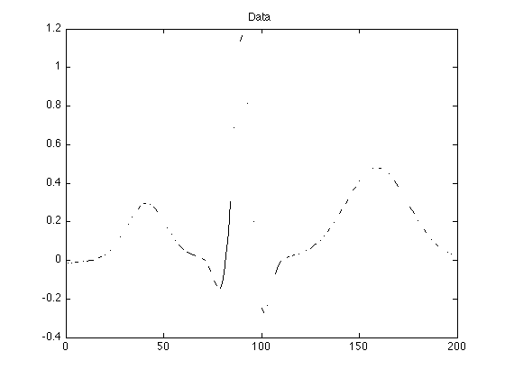
Display data
The NaN's appear as gaps in the plot
figure(1)
clf
plot(n, y)
title('Data')
Define matrix D
D represents the second-order derivitive (2nd-order difference). D is defined as a sparse matrix so that Matlab subsequently uses fast solvers for banded systems.
e = ones(N, 1);
D = spdiags([e -2*e e], 0:2, N-2, N);
Fist corner of D:
full(D(1:5, 1:5))
ans =

     1    -2     1     0     0
     0     1    -2     1     0
     0     0     1    -2     1
     0     0     0     1    -2
     0     0     0     0     1
Last corner of D:
full(D(end-4:end, end-4:end))
ans =

     1     0     0     0     0
    -2     1     0     0     0
     1    -2     1     0     0
     0     1    -2     1     0
     0     0     1    -2     1
Define matrices S and Sc
k = isfinite(y);                    % k : logical vector, indexes known values

S = speye(N);
S(~k, :) = [];                      % S : sampling matrix

Sc = speye(N);                      % Sc : complement of S
Sc(k, :) = [];

L = sum(~k)                         % L : number of missing values
L =

   100
Estimate missing data
Least square estimation of missing data. Note that the system matrix is banded so the system equations can be solved very efficiently with a fast banded system solver. By defining S and D as sparse matrices, Matlab calls a fast banded system solver by default.
v = -(Sc * (D' * D) * Sc') \ ( Sc * D' * D * S' * y(k)); % v : estimated samples
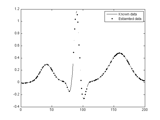
Fill in unknown values
Place the estimated samples into the signal.
x = zeros(N,1);
x(k) = y(k);
x(~k) = v;

% The above 3 lines is a more direct way to implement:
% x = Sc' * v + S'*y(k);

figure(1)
clf
plot(n, y, 'k', n(~k), x(~k) ,'k.')
legend('Known data', 'Estiamted data')
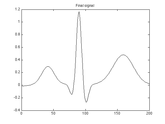
figure(1)
clf
plot(n, x )
title('Final signal')
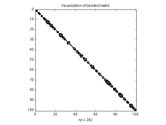
Banded matrix visualization
As noted above, the system matrix is banded. This can be visualized with the 'spy' command in Matlab:
G = Sc * (D' * D) * Sc';

figure(1)
clf
spy(G)
title('Visualization of banded matrix')

% It can be seen that all the non-zero elements of G lie near the diagonal.