Least square deconvolution

This example illustrates devonvolution using least squares

Ivan Selesnick
selesi@poly.edu

Start
Create data
Output data
Convolution matrix H
Direct solve (fails)
Diagonal loading (noise-free)
Diagonal loading (noisy)
Derivative regularization (noisy)

Start

clear
close all

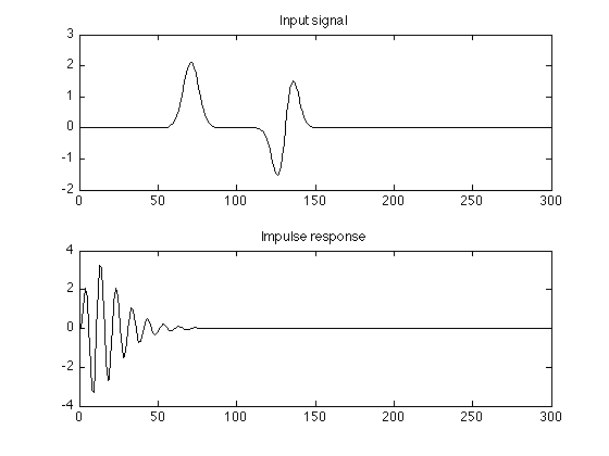
Create data

N = 300;
n = (0:N-1)';                               % n : discrete-time index

w = 5;
n1 = 70;
n2 = 130;
x = 2.1 * exp(-0.5*((n-n1)/w).^2) - 0.5*exp(-0.5*((n-n2)/w).^2).*(n2 - n);    % x : input signal

h = n .* (0.9 .^n) .* sin(0.2*pi*n);        % h : impulse response


figure(1)
clf
subplot(2, 1, 1)
plot(x)
title('Input signal');
YL1 = [-2 3];
ylim(YL1);

subplot(2, 1, 2)
plot(h)
title('Impulse response');

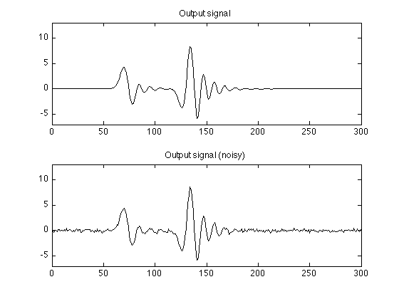
Output data

randn('state', 0);                          % Set state for reproducibility

y = conv(h, x);
y = y(1:N);                                 % y : output signal (noise-free)

yn = y + 0.2 * randn(N, 1);                 % yn : output signal (noisy)

figure(2)
clf
subplot(2, 1, 1)
plot(y);
YL2 = [-7 13];
ylim(YL2);
title('Output signal');

subplot(2, 1, 2)
plot(yn);
title('Output signal (noisy)');
ylim(YL2);

Convolution matrix H

Create convolution matrix H and verify that H*x is the same as y

H = convmtx(h, N);
H = H(1:N, :);                              % H : convolution matrix

% Verify that H*x is the same as y
e = y - H * x;   % should be zero
max(abs(e))

ans =

     0

Direct solve (fails)

Attempting to solve H*x = y leads to a solution of all NaN's (not a number)

g = H \ y;

%  H is singular

Warning: Matrix is singular to working precision.

g(1:10)

ans =

   NaN
   NaN
   NaN
   NaN
   NaN
   NaN
   NaN
   NaN
   NaN
   NaN

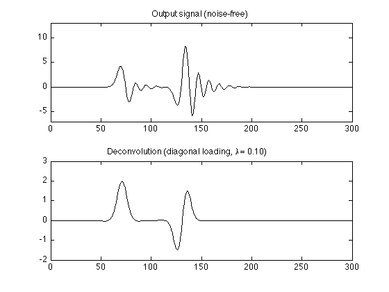
Diagonal loading (noise-free)

Diagonal overcomes the singularity of H.

lam = 0.1;
g = (H'*H + lam * eye(N)) \ (H' * y);

figure(1)
clf
subplot(2, 1, 1)
plot(y);
YL2 = [-7 13];
ylim(YL2);
title('Output signal (noise-free)');

subplot(2, 1, 2)
plot(g)
ylim(YL1);
title(sprintf('Deconvolution (diagonal loading, \\lambda = %.2f)', lam));

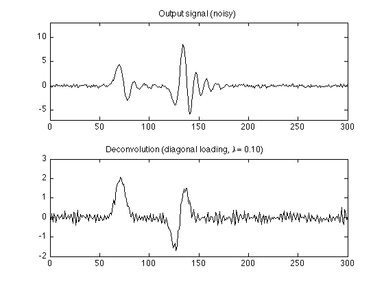
Diagonal loading (noisy)

lam = 0.1;
g = (H'*H + lam * eye(N)) \ (H' * yn);

figure(1)
clf
subplot(2, 1, 1)
plot(yn);
title('Output signal (noisy)');
ylim(YL2);

subplot(2, 1, 2)
plot(g)
title(sprintf('Deconvolution (diagonal loading, \\lambda = %.2f)', lam));

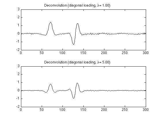
lam = 1.0;
g = (H'*H + lam * eye(N)) \ (H' * yn);

figure(2)
clf
subplot(2, 1, 1)
plot(g)
ylim(YL1)
title(sprintf('Deconvolution (diagonal loading, \\lambda = %.2f)', lam));

lam = 5.0;
g = (H'*H + lam * eye(N)) \ (H' * yn);

subplot(2, 1, 2)
plot(g)
ylim(YL1)
title(sprintf('Deconvolution (diagonal loading, \\lambda = %.2f)', lam));

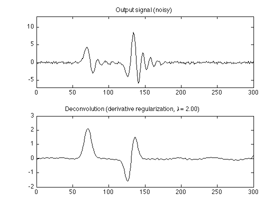
Derivative regularization (noisy)

e = ones(N, 1);
D = spdiags([e -2*e e], 0:2, N-2, N);       % second-order difference

First corner of D

full(D(1:5, 1:5))

ans =

     1    -2     1     0     0
     0     1    -2     1     0
     0     0     1    -2     1
     0     0     0     1    -2
     0     0     0     0     1

Last corner of D

full(D(end-4:end, end-4:end))

ans =

     1     0     0     0     0
    -2     1     0     0     0
     1    -2     1     0     0
     0     1    -2     1     0
     0     0     1    -2     1

Solve least squares problem

lam = 2.0;
g = (H'*H + lam * (D'*D)) \ (H' * yn);

figure(1)
clf
subplot(2, 1, 1)
plot(yn);
title('Output signal (noisy)');
ylim(YL2);

subplot(2, 1, 2)
plot(g)
title(sprintf('Deconvolution (derivative regularization, \\lambda = %.2f)', lam));