Example: Basis pursuit (BP) with the DFT

Sparse representation of complex sinusoids using basis pursuit (BP) with zero-padded DFT.

Contents

Misc

clear
close all

I = sqrt(-1);

Make signal

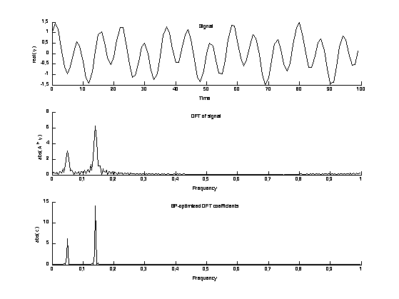
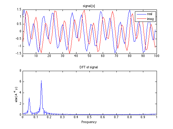
N = 100;                   % N : signal length
n = 0:N-1;

f1 = 0.05;
f2 = 0.14;
y = 0.5*exp(I*2*pi*f1*n) + exp(I*(2*pi*f2*n - pi/3));
% y : complex sinusoid

Define transform

Oversampled DFT

Nfft = 256;                 % Nfft : FFT length (including zero-padding)

[A, AH, normA] = MakeTransforms('DFT', N, Nfft);

Reconstruction error = 0.000000
Energy ratio = 1.000000

Display signal and its DFT

f = (0:Nfft-1)/Nfft;        % f : frequency axis

figure(1)
clf

subplot(2, 1, 1)
plot(n, real(y), n, imag(y), 'r')
legend('real','imag')
title('signal [s]')

subplot(2, 1, 2)
plot(f, abs( AH(y) ))
title('DFT of signal')
ylabel('abs( A^H y )')
xlabel('Frequency')

Solve BP problem

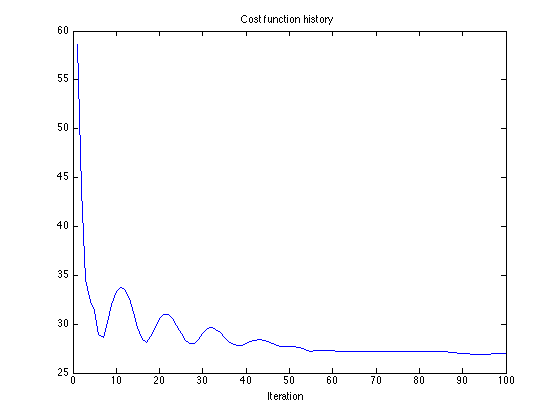
mu = 0.2;
Nit = 100;

[c, cost] = BP(y, A, AH, 1, mu, Nit);

% Display cost function history to observe convergence of algorithm.
figure(1)
clf
plot(cost)
title('Cost function history')
xlabel('Iteration')

Verify sparse coefficients

Verify that y = A(c); i.e., c is an exact representation of y.

RE = max(abs( y - A(c) ));

fprintf('Reconstruction error: %e\n', RE);

Reconstruction error: 1.443290e-15

Display

MyGraphPrefs('on')

figure(3)
clf

subplot(3, 1, 1)
% plot(n, real(y), n, imag(y), 'r')
% legend('real','imag')
line(n, real(y));
mytitle('Signal');
xlabel('Time')
ylabel('real( y )')

subplot(3, 1, 2)
line(f, abs(AH(y) ))
mytitle('DFT of signal');
ylabel('abs( A^H y )')
xlabel('Frequency')
box off

subplot(3, 1, 3)
line(f, abs(c), 'marker', '.')
mytitle('BP-optimized DFT coefficients');
ylabel('abs( c )')
xlabel('Frequency')


% print figure to pdf file
orient tall
print -dpdf figures/BP_example_dft_cplx

% print figure to eps file
set(gcf, 'PaperPosition', [1 1 4 5])
print -deps figures_eps/BP_example_dft_cplx

MyGraphPrefs('off')

Published with MATLAB® 7.12