Example: Basis pursuit denoising (BPD) with the STFT (with complex data)

Estimation of pulse in complex white Gaussian noise. The STFT is used.

Contents

Misc

clear
close all

I = sqrt(-1);

dB = @(x) 20 * log10(abs(x));

Make signal

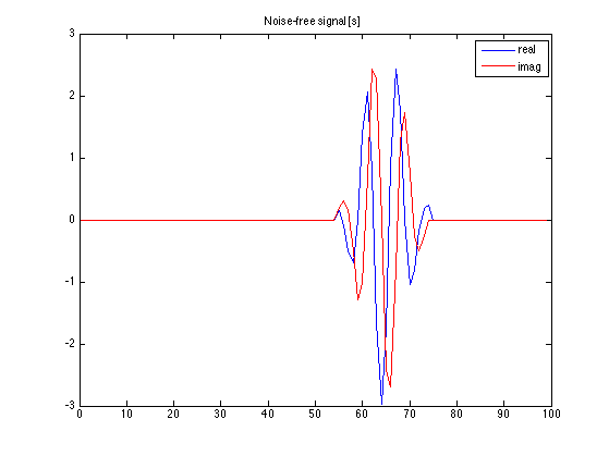
N = 100;                   % N : signal length
n = 0:N-1;

f = 0.15;
K = 20;                    % K : duration of pulse
M = 55;                    % M : start-time of pulse
A = 3;
s = zeros(size(n));
s(M+(1:K)) = A*exp(I*2*pi*f*(1:K)) .* hamming(K)';
% s : complex pulse

figure(1)
clf
plot(n, real(s), n, imag(s), 'r')
legend('real','imag')
title('Noise-free signal [s]')

Define transform

R = 16;         % R : frame length
Nfft = 32;      % Nfft : FFT length in STFT (Nfft >= R)

[A, AH, normA] = MakeTransforms('STFT', N, [R Nfft]);

Reconstruction error = 0.000000
Energy ratio = 1.000000

Make noisy data

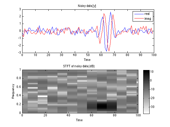
randn('state', 0); % set state for reproducibility of example

sigma = 0.5;
y = s + sigma * (randn(size(s)) + sqrt(-1)*randn(size(s))) / sqrt(2);

Display noisy data and its STFT

figure(1)
clf

subplot(2, 1, 1)
plot(n, real(y), n, imag(y), 'r')
legend('real','imag')
title('Noisy data [y]')
xlabel('Time')


AHy = AH(y);

tt = R/2 * ( (0:size(AHy, 2)) - 1 );    % tt : time axis for STFT

subplot(2, 1, 2)
imagesc(tt, [0 1], dB(AHy), max(dB(AHy(:))) + [-50 0])
axis xy
xlim([0 N])
ylim([0 1])
title('STFT of noisy data (dB)')
ylabel('Frequency')
xlabel('Time')
colorbar;

cm = colormap(gray);                    % cm : colormap for STFT
cm = cm(end:-1:1, :);
colormap(cm)

Solve BPD

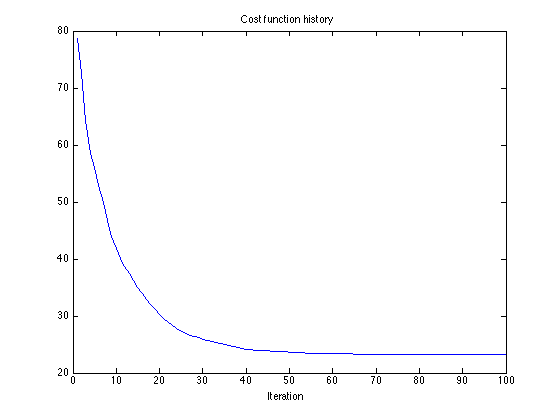
beta = 3;
lam = beta * sigma * normA;

mu = 0.1;
Nit = 100;

[c, cost] = BPD(y, A, AH, lam, mu, Nit);

x = A(c);

% Display cost function history to observe convergence of algorithm.
figure(1)
clf
plot(cost)
title('Cost function history')
xlabel('Iteration')

Display denoised signal

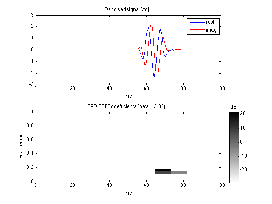
cmax = max(abs(c(:)));

figure(1)
clf

subplot(2, 1, 1)
plot(n, real(x), n, imag(x), 'r')
legend('real','imag')
title('Denoised signal [Ac]')
xlabel('Time')
ch = colorbar;
set(ch, 'visible', 'off')

subplot(2, 1, 2)
imagesc(tt, [0 1], dB(c), dB(cmax) + [-50 0])
axis xy
xlim([0 N])
ylim([0 1])
title(sprintf('BPD STFT coefficients (beta = %.2f)', beta));
ylabel('Frequency')
xlabel('Time')
colormap(cm)
ch = colorbar;
set(get(ch, 'title'), 'string', 'dB')

Optimality scatter plot

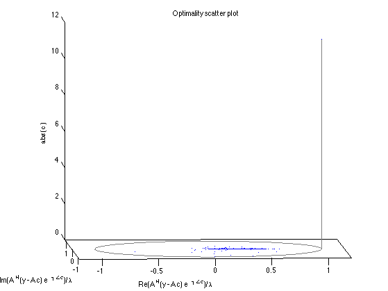
g = (1/lam) * AH(y - A(c)) .* exp(-I*angle(c));

figure(2)
clf
plot3( real(g(:)), imag(g(:)), abs(c(:)), '.')
zlabel('abs( c )')
xlabel('Re(A^H(y - A c) e^{-j\anglec})/\lambda')
ylabel('Im(A^H(y - A c) e^{-j\anglec})/\lambda')
title('Optimality scatter plot')
grid off
theta = linspace(0, 2*pi, 200);
line( cos(theta), sin(theta), 'color', [1 1 1]*0.5)
line([1 1], [0 0], [0 cmax],  'color', [1 1 1]*0.5)
xm = 1.2;
xlim([-1 1]*xm)
ylim([-1 1]*xm)
line([-1 1]*xm, [1 1]*xm, 'color', 'black')
line([1 1]*xm, [-1 1]*xm, 'color', 'black')

% Animate: vary view orientation
az = -36;
for el = [40:-1:5]
    view([az el])
    drawnow
end
for az = [-36:-3]
    view([az el])
    drawnow
end

Save figure to file

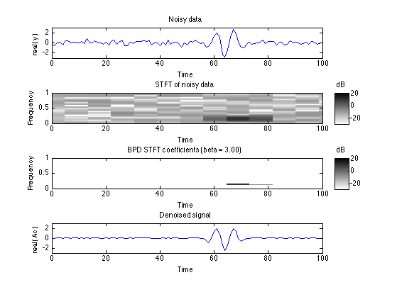
figure(1)
clf

subplot(4, 1, 1)
plot(n, real(y))
title('Noisy data');
ylabel('real( y )')
xlabel('Time')
ylim([-3 3])
ch = colorbar;
set(ch, 'visible', 'off')

subplot(4, 1, 2)
imagesc(tt, [0 1], dB(abs(AH(y))), dB(cmax) + [-50 0])
axis xy
colormap(cm)
xlim([0 N])
ylim([0 1])
ch = colorbar;
set(get(ch, 'title'), 'string', 'dB')
title('STFT of noisy data');
xlabel('Time')
ylabel('Frequency')

subplot(4, 1, 3)
imagesc(tt, [0 1], dB(c), dB(cmax) + [-50 0])
axis xy
colormap(cm)
xlim([0 N])
ylim([0 1])
ch = colorbar;
set(get(ch, 'title'), 'string', 'dB')
title(sprintf('BPD STFT coefficients (beta = %.2f)', beta));
xlabel('Time')
ylabel('Frequency')


subplot(4, 1, 4)
plot(n, real(A(c)))
title('Denoised signal');
ylabel('real( Ac )')
xlabel('Time')
ylim([-3 3])
ch = colorbar;
set(ch, 'visible', 'off')

orient tall
print -dpdf figures/BPD_example_stft_cplx

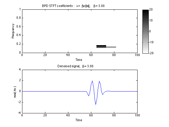
Animate: vary lambda

for beta = 0.1:0.1:3

    lam = beta * sigma * normA;
    [c, cost] = BPD(y, A, AH, lam, mu, Nit);
    x = A(c);

    figure(10)
    clf

    subplot(2, 1, 1)
    imagesc(tt, [0 1], dB(abs(c)), [-20 20])
    axis xy
    xlim([0 N])
    ylim([0 1])
    title(sprintf('BPD STFT coefficients : \\lambda = \\beta\\sigma ||a||, \\beta = %.2f', beta));
    ylabel('Frequency')
    xlabel('Time')
    colormap(cm)
    colorbar

    subplot(2, 1, 2)
    plot(n, real(x))
    ylim([-1 1]*4)
    title(sprintf('Denoised signal, \\beta = %.2f', beta));
    ylabel('real( Ac )')
    xlabel('Time')
    ch = colorbar;
    set(ch, 'visible', 'off')

    drawnow

end

Published with MATLAB® 7.12