TV denoising using convex and non-convex regularization

Ivan Selesnick selesi@nyu.edu Revised 2014, 2017

Contents

Start

clear

rmse = @(x) sqrt(mean(abs(x).^2));

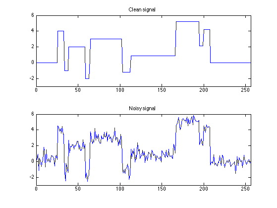
Create data

s = load('blocks.txt');          % blocks signal
y = load('blocks_noisy.txt');    % noisy blocks signal

sigma = 0.5;          % sigma : standard deviation of noise

N = length(s);        % N : length of signal

figure(1)
clf
subplot(2,1,1)
plot(s)
ax = [0 N -3 6];
axis(ax)
title('Clean signal');

subplot(2,1,2)
plot(y)
axis(ax)
title('Noisy signal');

TV Denoising

using L1 norm

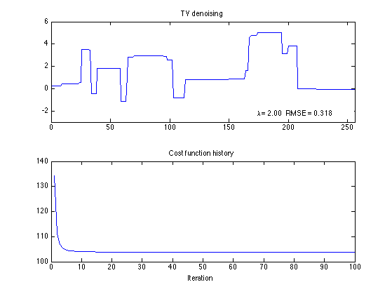
lam = 0.25 * sqrt(N) * sigma

Nit = 100;
[x_L1, cost] = tvd_mm(y, lam, Nit);

rmse_L1 = rmse(x_L1 - s);
txt_L1 = sprintf('\\lambda = %.2f   RMSE = %.3f', lam, rmse_L1);

figure(1)
clf
subplot(2,1,1)
plot(x_L1)
axis(ax)
title('TV denoising');
axnote(txt_L1)

subplot(2,1,2)
plot(cost)
title('Cost function history');
xlabel('Iteration')

lam =

     2

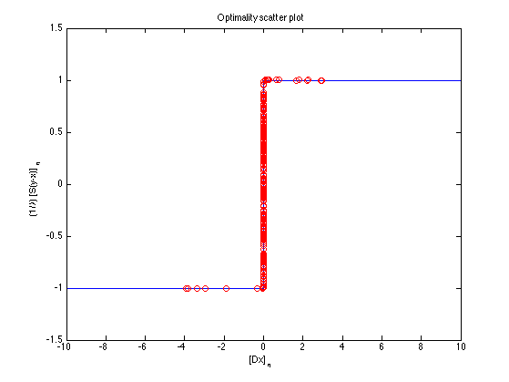
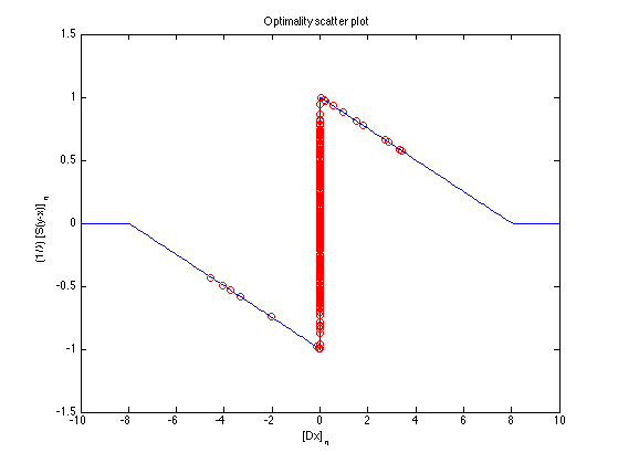
Optimality scatter plot

z = cumsum( x_L1 - y ) / lam;

figure(1)
clf
m = 10;
plot([-m 0 0 m], [-1 -1 1 1], diff(x_L1), z(1:end-1), 'o')
xlim([-m m])
ylim([-1.5 1.5])
ylabel('(1/\lambda) [S(y-x)]_n')
xlabel('[Dx]_n')
title('Optimality scatter plot')

Verify tvd_ncvx function

The (convex) TV solution is retrieved when the 'L1' option is used in the tvd_ncvx function.

[x_, cost_] = tvd_ncvx_ver1(y, lam, 'L1', Nit);

max(abs(x_L1 - x_))     % is zero
max(abs(cost - cost_))  % is zero

ans =

     0


ans =

     0

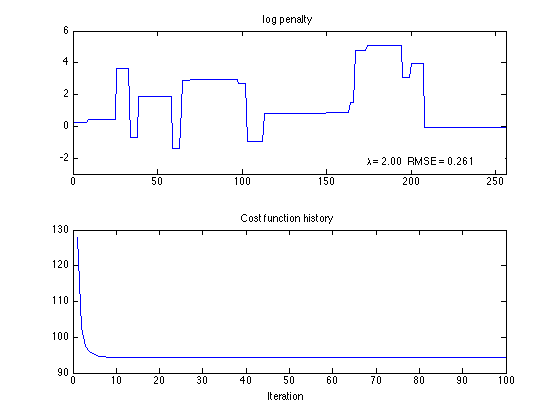
TV denoising using log penalty

[x_log, cost_log] = tvd_ncvx_ver1(y, lam, 'log', Nit);

rmse_log = rmse(x_log - s);
txt_log = sprintf('\\lambda = %.2f   RMSE = %.3f', lam, rmse_log);

figure(1)
clf
subplot(2,1,1)
plot(x_log)
axis(ax)
title('log penalty');
axnote(txt_log)

subplot(2,1,2)
plot(cost_log)
title('Cost function history');
xlabel('Iteration')

Optimality

z = cumsum( x_log - y ) / lam;

a = 1/(4*lam);    % maximal value for convexity
[phi, dphi, wfun, ds] = penalty_funs('log', a);

figure(1)
clf
m = 10;
t = [linspace(-m, -eps, 100) linspace(eps, m, 100)];
plot(t, dphi(t), diff(x_log), z(1:end-1), 'o');
xlim([-m m])
ylim([-1.5 1.5])
ylabel('(1/\lambda) [S(y-x)]_n')
xlabel('[Dx]_n')
title('Optimality scatter plot')

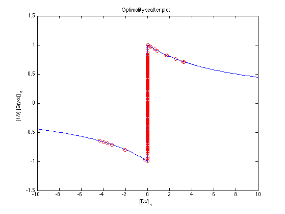
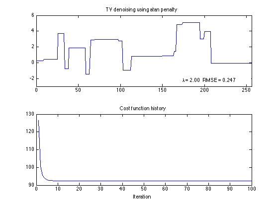
TV denoising using atan penalty

[x_atan, cost_atan] = tvd_ncvx_ver1(y, lam, 'atan', Nit);

rmse_atan = rmse(x_atan - s);
txt_atan = sprintf('\\lambda = %.2f   RMSE = %.3f', lam, rmse_atan);

figure(1)
clf
subplot(2,1,1)
plot(x_atan)
axis(ax)
title('TV denoising using atan penalty');
axnote(txt_atan)

subplot(2,1,2)
plot(cost_atan)
title('Cost function history');
xlabel('Iteration')

Optimality

z = cumsum( x_atan - y ) / lam;

a = 1/(4*lam);    % maximal value for convexity
[phi, dphi, wfun, ds] = penalty_funs('atan', a);

figure(1)
clf
m = 10;
t = [linspace(-m, -eps, 100) linspace(eps, m, 100)];
plot(t, dphi(t), diff(x_atan), z(1:end-1), 'o')
xlim([-m m])
ylim([-1.5 1.5])
ylabel('(1/\lambda) [S(y-x)]_n')
xlabel('[Dx]_n')
title('Optimality scatter plot')

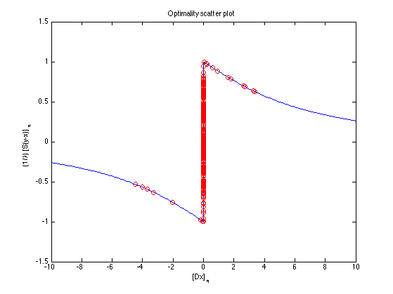
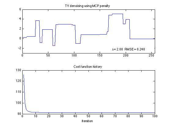
TV denoising using MC penalty

[x_mcp, cost_mcp] = tvd_ncvx_ver1(y, lam, 'mcp', Nit);

rmse_mcp = rmse(x_mcp - s);
txt_mcp = sprintf('\\lambda = %.2f   RMSE = %.3f', lam, rmse_mcp);

figure(1)
clf
subplot(2,1,1)
plot(x_mcp)
axis(ax)
title('TV denoising using MCP penalty');
axnote(txt_mcp)

subplot(2,1,2)
plot(cost_mcp)
title('Cost function history');
xlabel('Iteration')

Optimality

z = cumsum( x_mcp - y ) / lam;

a = 1/(4*lam);    % maximal value for convexity
[phi, dphi, wfun, ds] = penalty_funs('mcp', a);

figure(1)
clf
m = 10;
t = [linspace(-m, -eps, 100) linspace(eps, m, 100)];
plot(t, dphi(t), diff(x_mcp), z(1:end-1), 'o')
xlim([-m, m])
ylim([-1.5 1.5])
ylabel('(1/\lambda) [S(y-x)]_n')
xlabel('[Dx]_n')
title('Optimality scatter plot')

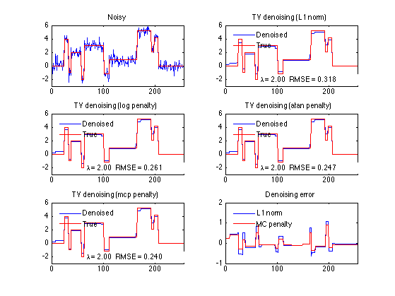
summary

n = 0:N-1;

figure(1)
clf

subplot(3, 2, 1)
plot(n, y, n, s)
axis(ax)
title('Noisy')

subplot(3, 2, 2)
plot(n, x_L1, n, s)
legend('Denoised', 'True', 'location', 'northwest')
legend boxoff
axis(ax)
title('TV denoising (L1 norm)');
axnote(txt_L1)

subplot(3, 2, 3)
plot(n, x_log, n, s)
legend('Denoised', 'True', 'location', 'northwest')
legend boxoff
axis(ax)
title('TV denoising (log penalty)');
axnote(txt_log)

subplot(3, 2, 4)
plot(n, x_atan, n, s)
legend('Denoised', 'True', 'location', 'northwest')
legend boxoff
axis(ax)
title('TV denoising (atan penalty)');
axnote(txt_atan)

subplot(3, 2, 5)
plot(n, x_mcp, n, s)
legend('Denoised', 'True', 'location', 'northwest')
legend boxoff
axis(ax)
title('TV denoising (mcp penalty)');
axnote(txt_mcp)

subplot(3, 2, 6)
plot(1:N, x_L1 - s, 1:N, x_mcp - s)
legend('L1 norm', 'MC penalty', 'location', 'northwest')
legend boxoff
xlim([0 N])
title('Denoising error')

orient landscape
print -dpdf Example1

Verify that version 1 and version 2 give the same output signal

penalty_list = {'log', 'atan', 'mcp'};

for i = 1:numel(penalty_list)

    pen = penalty_list{i};

    [x1, cost1] = tvd_ncvx_ver1(y, lam, pen, Nit); % Algorithm 1
    [x2, cost2] = tvd_ncvx_ver2(y, lam, pen, Nit); % Algorithm 2

    % Both algorithms give almost the same output signal.
    % (Using more iterations leads to more similar output signals.)
    max(abs(x1 - x2))

    figure(i)
    clf
    plot(1:Nit, cost1, 1:Nit, cost2)
    title(sprintf('TV denoising cost function history [%s penalty]', pen))
    legend('Algorithm 1', 'Algorithm 2')
end

ans =

    0.0038


ans =

    0.0034


ans =

    0.0030

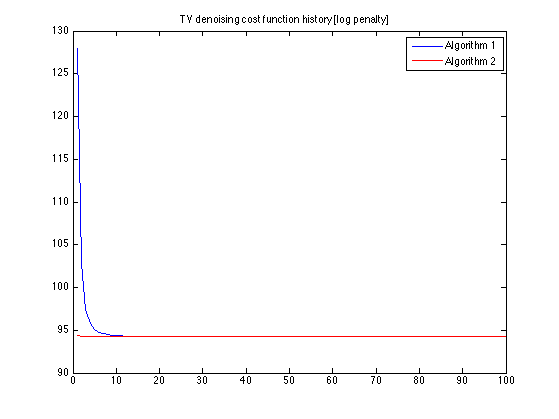
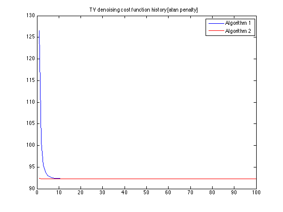
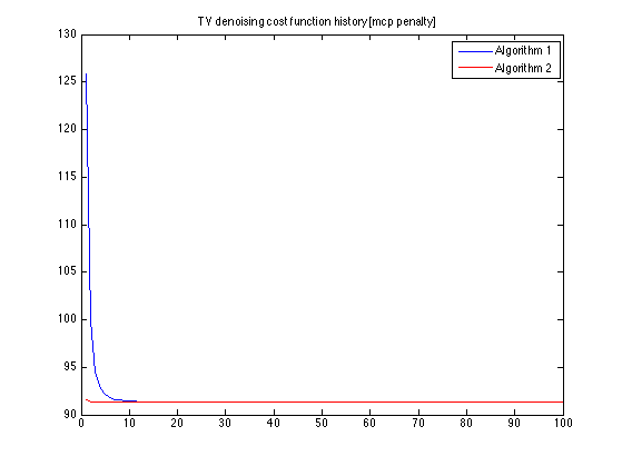
It can be seen that Algorithm 2 converges in fewer iterations than Algorithm 1.

Published with MATLAB® 7.12