Framelet2X: A Symmetric Framelet ToolBox
Research supported by ONR grant N000140310217
Introduction
We have developed a MATLAB ToolBox, Framelet2X, to accompany the paper:
I. W. Selesnick and A. Farras Abdelnour. Symmetric wavelet tight frames with two generators. Applied and Computational Harmonic Analysis, 17(2):211-225, September 2004. (Special Issue: Frames in Harmonic Analysis, Part II.)
The ToolBox contains programs to implement a particular type of over-complete (expansive) wavelet transform. We call this expansive transform a double-density discrete wavelet transform (DDWT) because it has exactly twice the number of wavelet coefficients as the critically-sampled DWT. The inverse transform is the transpose of the forward transform, and therefore it satisfies Parseval's energy property (the frame is 'tight').
The programs in the ToolBox implement symmetric boundary conditions. The implementation satisfies Parseval's energy property. These notes describe the implementation of the transform and verifies its properties.
We use cell arrays in MATLAB to store the wavelet coefficients because it simplifies the programs and it also makes it easy to access the wavelet coefficients corresponding to a specific scale. A cell array can be used to store a set of vectors, each vector having possibly different lengths. Because there are a different number of wavelet coefficients at each scale, a cell array is convenient for organizing the wavelet coefficients.
The MATLAB Programs
| filters1.m | filter coefficients (Example 1 in the paper) |
| afb.m | analysis filter bank |
| sfb.m | synthesis filter bank |
| ddwt.m | double-density wavelet transform |
| ddwti.m | inverse double-density wavelet transform |
| up.m | upsampling |
| check.m | check PR, symmetric extension, etc. |
Download the Framelet2X MATLAB ToolBox
The zip file, Framelet2X.zip, contains the programs listed above. It also contains MATLAB programs to generate the af filter coefficients (example 1 in the paper).The Filters
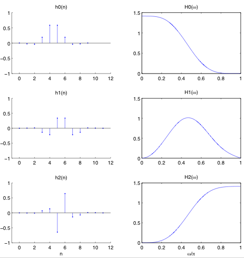
The analysis filters are stored as the cell array af, and the synthesis filters are stored as the cell array sf. Because the frame is a tight frame, the synthesis filters are the time-reversed versions of the analysis filters. The filter af{1} is the symmetric even-length lowpass filter, the filter af{2} is the symmetric even-length bandpass filter, and the filter af{3} is the anti-symmetric even-length highpass filter.
We can create the following plots of the impulse responses and frequency responses of the three filters with the MATLAB code contained in the accompanying file check.m.
Checking the Perfect Reconstruction Conditions
We can check the perfect reconstruction (PR) conditions using the following code fragment. The perfect reconstruction conditions are equations (3) and (4) in the paper:
H0(z) H0(1/z) + H1(z) H1(1/z) + H2(z) H2(1/z) = 2
H0(-z) H0(1/z) + H1(-z) H1(1/z) + H2(-z) H2(1/z) = 0
% check perfect reconstruction conditons

[af, sf] = filters1;
h0 = [af{1}; 0; 0];
h1 = af{2};
h2 = af{3};

N = length(h0);
n = [0:N-1]';

g0 = h0(N-n);
g1 = h1(N-n);
g2 = h2(N-n);

Eq3 = conv(h0,g0) + conv(h1,g1) + conv(h2,g2);

s = (-1).^n;
f0 = h0 .* s;
f1 = h1 .* s;
f2 = h2 .* s;

Eq4 = conv(f0,g0) + conv(f1,g1) + conv(f2,g2);

[Eq3 Eq4]
The result of running this program is the following, which verifies that these filters do satisfy the PR conditions.
                  0                  0
                  0                  0
   0.00000000000000   0.00000000000000
  -0.00000000000000   0.00000000000000
  -0.00000000000000  -0.00000000000000
  -0.00000000000000  -0.00000000000000
   0.00000000000001   0.00000000000001
  -0.00000000000007   0.00000000000000
  -0.00000000000000   0.00000000000001
   0.00000000000036  -0.00000000000000
  -0.00000000000002  -0.00000000000000
   1.99999999999940   0.00000000000000
  -0.00000000000002   0.00000000000000
   0.00000000000036  -0.00000000000000
  -0.00000000000000  -0.00000000000001
  -0.00000000000007   0.00000000000000
   0.00000000000001  -0.00000000000001
  -0.00000000000000  -0.00000000000000
  -0.00000000000000   0.00000000000000
  -0.00000000000000   0.00000000000000
   0.00000000000000  -0.00000000000000
                  0                  0
                  0                  0
Implementing the Analysis and Synthesis Filter Banks
The basic building block of the double-density DWT is the analysis and synthesis filter banks. The analysis filter bank is implemented with the program afb. The program returns three subband signals obtained by filtering the input signal with each of three filters and down-sampling by two. The three subband signals are called lo, hi1, and hi2 in the afb program. In the implementation, there are a couple of details that must be taken into account. First, the symmetric extension at the boundaries of the signal requires that the input signal be symmetrically extended before the filtering is performed. While periodic extension at the boundaries is easier to implement than symmetric extension, periodic extensions give rise to undesirable artifacts at the boundaries of the reconstructed signal when the wavelet coefficients are processed. Since our filters are symmetric, we can perform symmetric extension. (Symmetric extension of the boundaries requires that the filters be symmetric.) It turns out that symmetric extension for the symmetric double-density DWT filters is not as straightforward as it is for the symmetric biorthogonal DWT. That is because the even-length symmetric biorthogonal filters are symmetric and anti-symmetric about the same point. However, the filters for the double-density DWT are symmetric about different points. It turns out that for the double-density DWT with symmetric extension, the bandpass and highpass subbands will have a different number of samples each. If the input signal x has length N (with N even) then one would expect that each of the three subband signals will be of length N/2. When implementing the symmetric extension, the lowpass subband signal will have length N/2, however, the bandpass subband signal will have length N/2+1 and the highpass subband signal will have length N/2-1. So the total number of subband coefficients is 3N/2 as expected.
Second, in order to have Parseval's energy relation, it is necessary that the end-points of the bandpass subband signal be normalized (divided) by sqrt(2). In the synthesis filter bank, this normalization is removed by multiplying those endpoints by sqrt(2). This normalization is not needed to have the perfect reconstruction property, it is only needed to satisfy Parseval's energy relation exactly. (That the energy of the signal can be computed by the sum of the energies of the subband signals.).
The synthesis filter bank is implemented with the program sfb.
We can check the perfect reconstruction conditions using the following MATLAB code fragment:
>> [af, sf] = filters1;
>> x = rand(1,64);
>> [lo, hi1, hi2] = afb(x, af);
>> y = sfb(lo, hi1, hi2, sf);
>> err = x - y;
>> max(abs(err))

ans =

     2.909894547542535e-13
Parseval's Energy Relation
We can check Parseval's energy relation with the following MATLAB code fragment:
>> x*x'

ans =

  20.52511996979790

>> lo*lo' + hi1*hi1' + hi2*hi2'

ans =

  20.52511996979641
This illustrates that the total energy of the three subband signals equals the energy of the input signal.
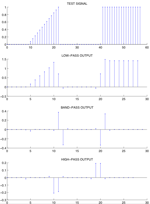
For a simple test signal the following figure illustrates the three subband signals. Notice that the bandpass and highpass subbands signals equal zero over the constant and ramp segments of the test signal, except for neighborhoods around the discontinuities. This illustrates the vanishing moment properties of the filters.
Implementing the Double-Density DWT
The main program for computing the double-density DWT is ddwt. The program is very simple. It just calls the analysis filter bank program afb iteratively --- each time reassigning the input signal x as the lowpass subband signal and storing the bandpass and highpass subband signals in a cell array.
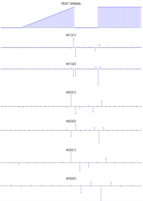
To clarify the way in which the wavelet coefficients are organized in the cell array, lets take a 3-level DDWT of a length 128 signal:
>> [af, sf] = filters1;
>> x = rand(1,128);
>> w = ddwt(x,3,af)

w =

    {1x2 cell}    {1x2 cell}    {1x2 cell}    [1x16 double]
The cell w{1} contains the wavelet coefficients coming from the first level.
>> w{1}

ans =

    [1x65 double]    [1x63 double]
The vector w{1}{1} contains the 65 wavelet coefficients coming from the bandpass subband at the first level, and w{1}{2} contains the 63 wavelet coefficients coming from the highpass subband at the first level. Similarly:
>> w{2}

ans =

    [1x33 double]    [1x31 double]

>> w{3}

ans =

    [1x17 double]    [1x15 double]
Parseval's Energy Relation
We can verify that the energy of the input signal and the total energy of the wavelet coefficients are equal using the following MATLAB code fragment.
>> [af, sf] = filters1;
>> x = rand(1,128);
>> E1 = x*x'

E1 =

   41.3498

>> w = ddwt(x,3,af);
>> E2 = sum(w{4}.^2);
>> for j = 1:3, for i = 1:2, E2 = E2 + sum(w{j}{i}.^2); end, end, E2

E2 =

   41.3498

>> E1 - E2

ans =

   8.1641e-12
The energy of the signal, E1, and the total energy in the wavelet domain, E2, are the same.
The program for the inverse double-density DWT is ddwti.
Using the program ddwti we can plot the wavelets by setting all the wavelet coefficients to zero, except for one of them at a time. Then, computing the inverse DDWT gives the corresponding wavelet.
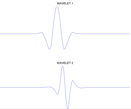
In the program check accompanying this document, the wavelets that coincide with the boundary of the signal are also shown, to illustrate the symmetric extension.
A Simple Test Signal
For a simple 128-point test signal, the following figure illustrates the wavelet coefficients of a 3-level double-density DWT.
For the N=128 point signal, the total number of wavelet coefficients is N + N/2 + N/4 + N/8 = 15 N/8 = 240.