Inverse system example

Given h, find g such that conv(h, g) = impulse

Start
Impulse response h
Poles of H(z)
Partial fraction expansion
Causal impulse response g
Stable impulse response g
Verify the inverse system
Example
Compute the output of H
Compute the output of G

Start

clear
close all

set(0, 'DefaultLineMarkerSize', 5)
set(0, 'DefaultLineMarkerFaceColor', 'black')

u = @(n) (n >= 0);
del = @(n) (n == 0);

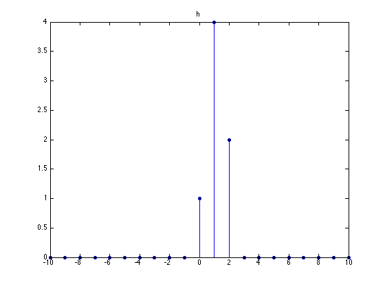
Impulse response h

n = -10:10;
h = del(n) + 4 * del(n-1) + 2 * del(n-2);

stem(n, h)
title('h')

Poles of H(z)

roots([1 4 2])

ans =

   -3.4142
   -0.5858

Partial fraction expansion

[r, p, k] = residue([1 0],[1 4 2])

r =

    1.2071
   -0.2071


p =

   -3.4142
   -0.5858


k =

     []

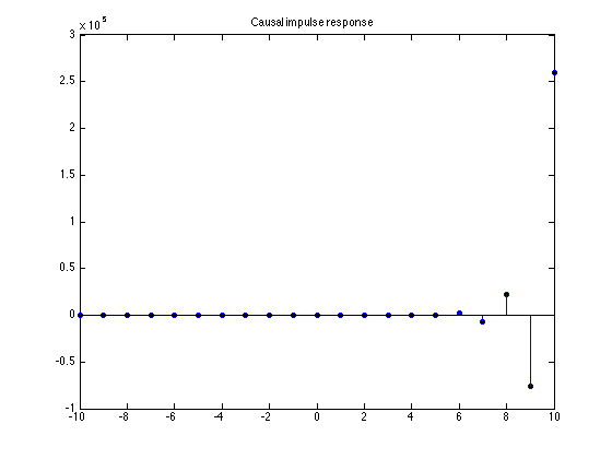
Causal impulse response g

This impulse response is causal but not stable! Note that the vertical axis goes up to 10^5

g = r(1) * p(1).^n .* u(n) + r(2) * p(2).^n .* u(n);

stem(n, g);
title('Causal impulse response')

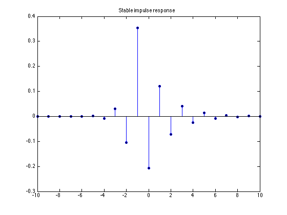
Stable impulse response g

This impulse response is stable but not causal

g = -r(1) * p(1).^n .* u(-n-1) + r(2) * p(2).^n .* u(n);

stem(n, g)
title('Stable impulse response')

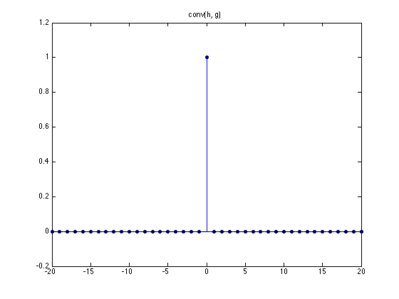
Verify the inverse system

Verify that the convolution of h and g is the impulse function

f = conv(h, g);

stem(f)
% In the plot, the impulse is at the wrong location.
% We need to specify the time axis.

% stem(n, f) causes an error because f is longer than n

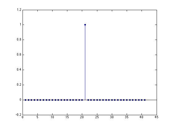
This validates the correctness of g

stem(-20:20, f)
% be aware of time axis when performing convolution

title('conv(h, g)')

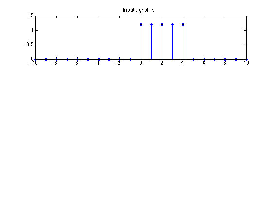
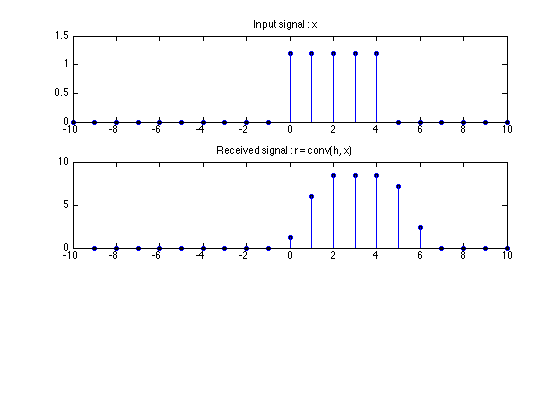
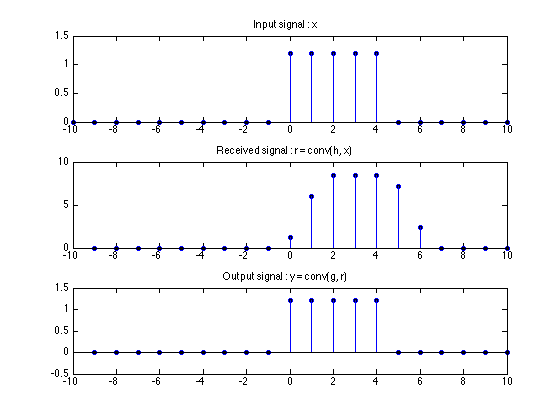
Example

x = 1.2*u(n) - 1.2*u(n-5);

subplot(3, 1, 1)
stem(n, x)
title('Input signal : x')

Compute the output of H

r = conv(h, x);

subplot(3, 1, 2)
stem(-20:20, r)
xlim([-10 10])
title('Received signal : r = conv(h, x)')

Compute the output of G

Observe that the output of G is the same as the input to H

y = conv(g, r);

subplot(3, 1, 3)
stem(-30:30, y)
xlim([-10 10])
title('Output signal : y = conv(g, r)')

set(0, 'DefaultLineMarkerSize', 'remove')
set(0, 'DefaultLineMarkerFaceColor', 'remove')