Computing the impulse response of a system with complex poles (Example 1)

This example shows three different ways to compute the impulse response.

Define system coefficients
Compute impulse response directly from different equation
Compute impulse response using partial fraction expansion
Compute impulse response using cosine formula
Plot all

Define system coefficients

Difference equation: y(n) = x(n) - 2.5 x(n-1) + y(n-1) - 0.7 y(n-2)

b = [1 -2.5];
a = [1 -1 0.7];

Compute impulse response directly from different equation

Use the MATLAB function 'filter' to compute the impulse response

u = @(n) n >= 0;     % step signal
del = @(n) n == 0;   % impulse signal

n = -10:30;
x = del(n);             % impulse
h1 = filter(b, a, x);   % impulse response

figure(1)
clf
stem(n, h1, 'filled');
title('Impulse response computed using difference equation')

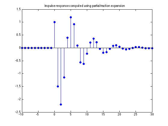
Compute impulse response using partial fraction expansion

Use MATLAB function 'residue' to find the poles and residues.

[r, p, k] = residue(b,a)

% r =
%    0.5000 + 1.4907i
%    0.5000 - 1.4907i
%
% p =
%    0.5000 + 0.6708i
%    0.5000 - 0.6708i
%
% k =
%      []


h2 = r(1)*p(1).^n .* u(n) + r(2)*p(2).^n .* u(n);

figure(1)
clf
stem(n, h2, 'filled')
title('Impulse response computed using partial fraction expansion')

r =

   0.5000 + 1.4907i
   0.5000 - 1.4907i


p =

   0.5000 + 0.6708i
   0.5000 - 0.6708i


k =

     []

Verify that h2 is the same as h1

max(abs(h1 - h2))
% This is zero to machine precision

ans =

   8.8818e-16

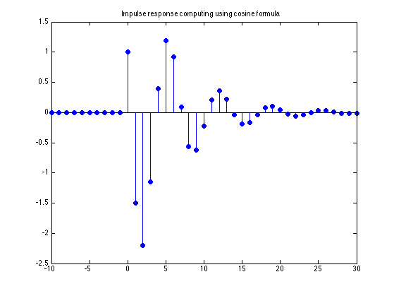
Compute impulse response using cosine formula

R = abs(r(1));
theta = angle(r(1));

a = abs(p(1));
om = angle(p(1));

h3 = 2 * R * a.^n .* cos(om * n + theta) .* u(n);

figure(1)
clf
stem(n, h3, 'filled')
title('Impulse response computing using cosine formula')

Verify that h3 is the same as h1

max(abs(h1 - h3))
% This is zero to machine precision

ans =

   9.8532e-16

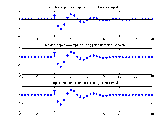
Plot all