Matlab demo: Frequency response
Illustrate frequency response concept and equations
Contents
Start
close all
clear
Define a system
% The system y(n) = 0.2 x(n) + 0.3 x(n-1) + 0.8 y(n-1)
% is represented by its coefficient vectors 'a' and 'b':
b = [0.2 0.3];
a = [1 -0.8];
Define a cosine
om1 = 0.09*pi;   % radians/sample

n = 0:100;
x = cos(om1 * n);

figure(1)
stem(n, x, '.')
ylim([-2 2])

% The frequency om1 is f1 = 0.045 cycles/sample.  f1 = om1/(2*pi).
% So, one cycle is 1/0.045 = 22.2 samples,
% which can be seen in the plot.
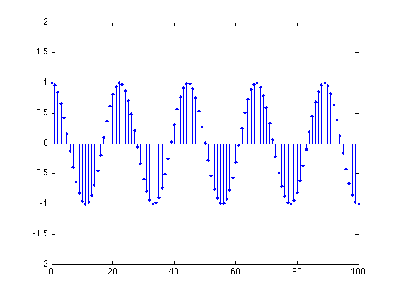
Compute system output
y = filter(b, a, x);

figure(1)
stem(n, y, '.')
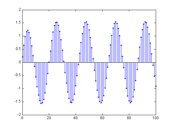
Evaluate H(om1)
z1 = exp(1j * om1);
Hom1 = (0.2*z1 + 0.3)/(z1 - 0.8);   % Value of frequency response at om1
abs(Hom1) % This is |H(om1)|
ans =

    1.5391
angle(Hom1) % This is the angle of H(om1)
ans =

   -0.9364
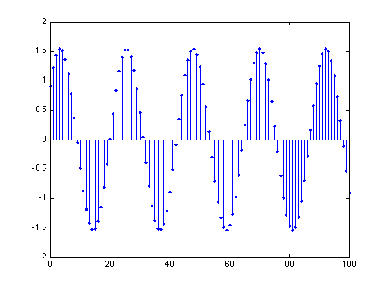
Formula for output
The output, as predicted by the frequency response formula, is:
p = abs(Hom1) * cos(om1 * n + angle(Hom1));

figure(1)
stem(n, p, '.')
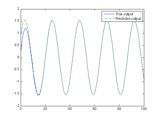
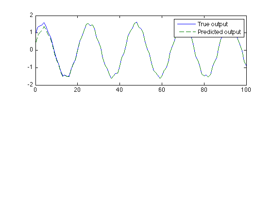
Plot both the true output and the predicted output signal to see if they agree
figure(1)
plot(n, y, n, p, '--')
legend('True output', 'Predicted output')

% Note: the predicted output is correct except for the transient.
% The formula is correct once _steady_state_ is reached.
Use freqz
The frequency response can be computed using the 'freqz' command.
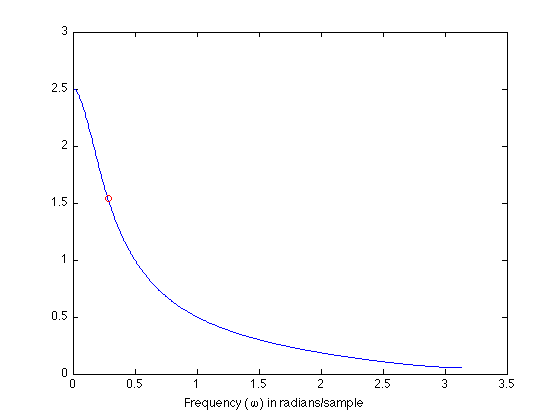
[H, om] = freqz(b, a);

figure(1)
plot(om, abs(H))
xlabel('Frequency (\omega) in radians/sample')

The value we computed for H(om1) should be consistent. We can check that H(om1) lies on this plot.
figure(1)
plot(om, abs(H), om1, abs(Hom1), 'ro')
xlabel('Frequency (\omega) in radians/sample')
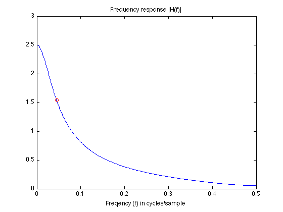
Plot using frequency in units of cycles/sample
figure(1)
plot(om/(2*pi), abs(H), om1/(2*pi), abs(Hom1), 'ro')
xlabel('Freqency (f) in cycles/sample')
title('Frequency response |H(f)|')
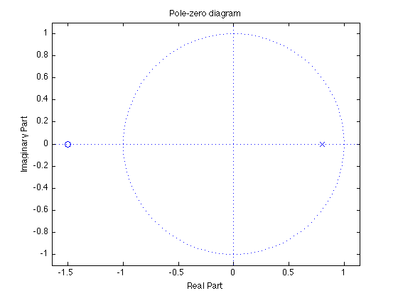
Pole/zero plot
figure(1)
zplane(b, a)
title('Pole-zero diagram')
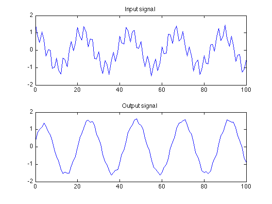
Two frequencies
Create a signal consisting of two cosines and compute the output of the system.
om2 = 0.6*pi;

x = cos(om1 * n) + 0.5 * cos(om2 * n);

y = filter(b, a, x);     % output of filter

figure(1)
subplot(2, 1, 1)
plot(n, x)
title('Input signal')

subplot(2, 1, 2)
plot(n, y)
title('Output signal')
Evaluate H(om2)
H(om1) is found already above. Now find H(om2)
z2 = exp(1j * om2);
Hom2 = (0.2*z2 + 0.3)/(z2 - 0.8);   % Value of frequency response at om2
Compare H(om1) and H(om2)
abs(Hom1)
% Note: |H(om1)| > 1 so the first cosine is _amplified_ by the system.
ans =

    1.5391
abs(Hom2)
% Note: |H(om2)| < 1 so the second cosine is _attenuated_ by the system.
ans =

    0.2086
Predict the output using the frequency response formula
p = abs(Hom1) * cos(om1 * n + angle(Hom1)) + 0.5 * abs(Hom2) * cos(om2 * n + angle(Hom2));

figure(1)
clf
subplot(2,1,1)
plot(n, p, n, y, '--')
legend('True output', 'Predicted output')

% The predicted output is valid in the steady state.
The transient?
Q: How long does it take for the system to reach steady state?
A: As long as it takes for the impulse response to diminish. Which depends on how close the pole is to the unit circle. The closer the pole is to the unit circle, the longer it takes for the impulse response to decay to zero.