Thresholding is a technique used for signal and image denoising. The discrete wavelet transform uses two types of filters: (1) averaging filters, and (2) detail filters. When we decompose a signal using the wavelet transform, we are left with a set of wavelet coefficients that correlates to the high frequency subbands. These high frequency subbands consist of the details in the data set. If these details are small enough, they might be omitted without substantially affecting the main features of the data set. Additionally, these small details are often those associated with noise; therefore, by setting these coefficients to zero, we are essentially killing the noise. This becomes the basic concept behind thresholding-set all frequency subband coefficients that are less than a particular threshold to zero and use these coefficients in an inverse wavelet transformation to reconstruct the data set.

After implementing the double-density DWT, and double-density complex DWT for 1-D signals, we can develop two different methods using these DWTs to remove noise from an image. The double-density DWT method will be discussed first.

1. 1-D Double-Density DWT Thresholding Method

function y = double_S1D(x,T)

% x: noise signal
% T: threshold

[af, sf] = filters1;
J = 4;
w = double_f1D(x,J,af);
% loop through scales
for j = 1:J
    % loop through subbands
    for s = 1:2
       w{j}{s} = soft(w{j}{s},T);
    end
end
y = double_i1D(w,J,sf);

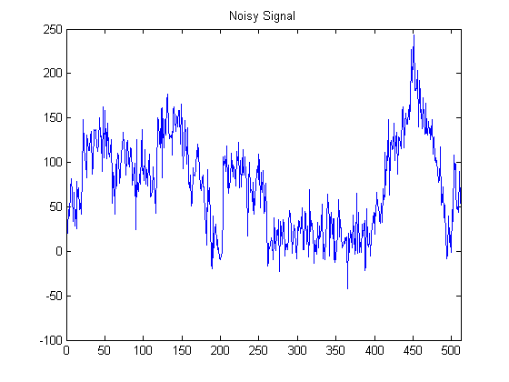
This program takes as input two parameters, one of which is the noisy input signal (to be thresholded) and the other of which is the threshold point. A sample noisy signal is shown below, whose length is 512. To denoise the signal, we first take the forward double-density DWT over four scales. Then a denoising method, knows as soft thresholding, is applied to the wavelet coefficients though all scales and subbands. The soft thresholding method sets coefficients with values less than the threshold T to 0, then subtracts T from the non-zero coefficients. After performing soft thresholding, we take the inverse wavelet transform of the new wavelet coefficients.

Figure 13.   Noisy 1-D Signal.

The following section of MATLAB code shows how to convert an image to a double data type (for compatibility with MATLAB), how to create a noisy signal, and display the denoised signal after applying the 1-D double-density DWT method. Note that we use a threshold value of 25, which is the optimal threshold point for this case. Later, we will illustrate how to find the optimal threshold value.

>> s1 = double(imread('peppers.jpg')); % load image as a double
>> s = s1(:,4,3);		       % convert 3-D image to a 1-D signal
>> subplot (3,1,1), plot(s)	       % plot the original signal
>> title('Original Signal')
>> x = s + 20*randn(size(s));	       % add Gaussian noise to the signal
>> subplot (3,1,2), plot(x)	       % plot the noisy signal
>> title('Noisy Signal')
>> T = 25;			       % choose a threshold of 20
>> y = double_S1D(x,T);		       % denoise the noisy signal using
                                       % double-density DWT
>> subplot(3,1,3), plot(y)	       % display the denoised signal
>> title('Denoised Signal')

The double-density DWT method results in the following denoised signal (Figure 9).

Figure 14.   Denoised Signal By Double-Density DWT Denoising Method.

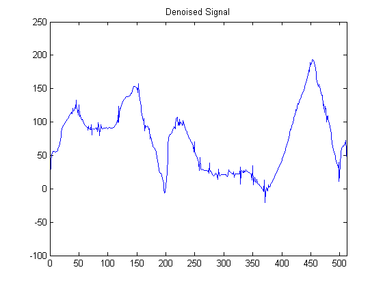
From the resulting image, we can see the denoising capability of the 1-D double-density DWT. We want to improve the effect by using the 1-D double-density dual-tree DWT. The optimal threshold for this procedure is 20. The MATLAB function doubledual_S1D.m and the resulting denoised image are shown below.

2. 1-D Double-Density Complex DWT Thresholding Method

function y = doubledual_S1D(x,T)

% x - noise signal
% T - threshold

[Faf, Fsf] = FSdoubledualfilt;
[af, sf] = doubledualfilt;
J = 4;
w = doubledualtree_f1D(x,J,Faf,af);
% loop thru scales:
for j = 1:J
    % loop thru subbands
    for s1 = 1:2
        for s2 = 1:2
            w{j}{s1}{s2} = soft(w{j}{s1}{s2},T);
        end
    end
end
y = doubledualtree_i1D(w,J,Fsf,sf);

The double-density complex DWT method results in the following denoised signal (Figure 10).

Figure 15.   Denoised Signal By Double-Density Complex DWT Denoising Method.

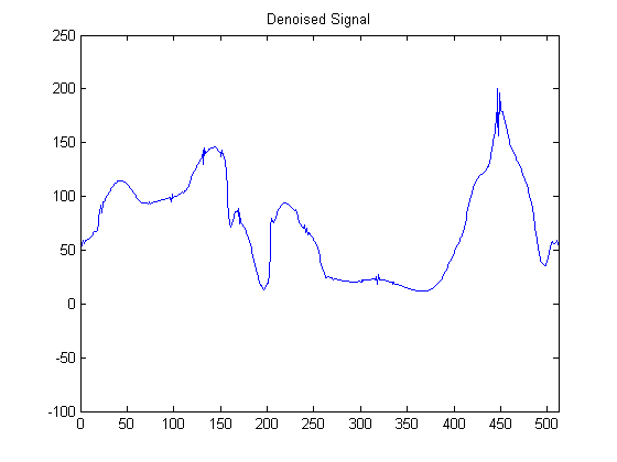
From the resulting image above, we can see the denoising capability of the 1-D double-density DWT. We can see that 1-D complex double-density method removes more noise signal than 1-D double-density method does. This can be proved by the "RMS Error vs. Threshold Point" plot, which is shown below.

Figure 16.   RMS Error vs. Threshold Point Comparison Between Double-Density DWT And Double-Density Complex DWT Denoising Methods.

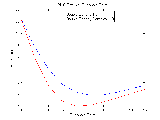
From Figure 11, we can also see where the optimal threshold point value lies. For each method, we would like the RMS error to be minimized. This will occur at the optimal threshold point value. By applying the optimal threshold point, we can produce the minimum RMS error and yield the optimal noise attenuation. From Figure 11, we can see the denoising capability for the two different methods, with double-density complex DWT method being the better of the two. The double-density DWT method can reduce the noise of a signal from 20 to about 8, whereas the double-density complex DWT method can reduce the noise of a signal from 20 to about 6. This is a notable improvement. The figure above was generated by the following code.

>> s1 = double(imread('peppers.jpg'));	% load image as a double
>> s = s1(:,2,3);			% convert to a 2-D image
>> x = s + 20*randn(size(s));		% add Gaussian noise to image
>> t = 0:5:45;         			% threshold range (0-45)
>> e = double_den1(s,x,t);    		% using double-density DWT &
>> de = double_dual1(s,x,t);  		% double-density dual-tree DWT
>> figure(1)
>> plot(t,e,'blue')			% plot double-density
>> hold on
>> plot(t,de,'red')			% plot double-density dual-tree
>> title('RMS Error vs. Threshold Point')
>> xlabel('Threshold Point');
>> ylabel('RMS Error');
>> legend('Double-Density 1-D','Double-Density Complex 1-D',0);

Summary of Programs:

1. double_S1D.m - 1-D double-density DWT denoising method
2. doubledual_S1D.m - 1-D double-density complex DWT denoising method
3. Example_SignalDenoising1.m - Signal denoising example using double-density DWT method
4. Example_SignalDenoising2.m - Signal denoising example using double-density complex DWT method
5. double_den1.m - Compute RMS error vs. threshold point for double-density DWT method
6. double_dual1.m - Compute RMS error vs. threshold point for double-density complex DWT method
7. Example_Compare1DThresholds.m - Plot RMS error vs. threshold point
8. soft.m - Soft thresholding