There are two versions of the 2-D double-density dual-tree DWT: (1) The 2-D double-density dual-tree real-oriented DWT, which is 2-times expansive, and (2) The 2-D double-density dual-tree complex-oriented DWT, which is 4-times expansive.

1. Real 2-D Double-Density Dual-Tree DWT

The 2-D double-density dual-tree real DWT of an image i is implemented by using two oversampled 2-D double-density DWTs in parallel. Then, for each pair of subbands, we take the sum and difference. The MATLAB program, doubledualtree_f2D.m computes the real 2-D double-density dual-tree DWT w of an image x.

The wavelet coefficients w are stored in a cell array data structure w{j}{k}{d}, for j = 1 - J, k = 1 - 2, and d = 1 - 8, where j represents the scale, and (k,d) represents the orientation. The image can be reconstructed using the doubledualtree_i2D.m MATLAB function. We ensure the perfect reconstruction condition is kept with the following code fragment.

>> x = rand(256);			% create generic 2-D test signal
>> J = 3;				% number of stages (3)
>> [Faf, Fsf] = FSdoubledualfilt;	% filters for first stage
>> [af, sf] = doubledualfilt;		% filters for remaining stages
>> w = doubledualtree_f2D(x, J, Faf, af);% analysis filters bank
>> y = doubledualtree_i2D(w, J, Fsf, sf);% synthesis filter bank
>> err = x - y; 			% compute error signal
>> max(max(abs(err)))			% verify that error is zero

ans =

  6.3827e-013

First, we generate a random 2-D input signal x of length 256. The analysis and synthesis filter bank is then computed first from the FSdoubledualfilt.m and doubledualfilt.m functions. The 3-scale forward double-density complex DWT is computed with the doubledualtree_f2D.m function to generate a function w. We then apply the inverse double-density complex DWT to this function using the doubledualtree_i2D.m MATLAB function. To ensure that the perfect reconstruction condition has been met, we then find the difference between the input signal x and the output signal y. As you can see, the differences found here are again significantly close to zero, and can actually be considered as zero.

function w = doubledualtree_f2D(x, J, Faf, af)

% Forward Real 2-D Double-Density Dual-Tree DWT
%
% USAGE:
%   w = doubledualtree_f2D(x, J, Faf, af)
% INPUT:
%   x - an image of size M x N
%   J - number of stages
%   Faf - analysis filters for first stage
%   af - analysis filters for remaining stages
% OUPUT:
%   w{j}{d1}{d2} - DWT coefficients
%       j = 1 - J, k = 1 - 2, d = 1 - 8
%   w{J+1}{k} - lowpass coefficients
%       k = 1 - 2

% normalization
x = x/sqrt(2);

% Tree 1
[x1 w{1}{1}] = afb3_2D(x, Faf{1});      % stage 1
for j = 2:J
    [x1 w{j}{1}] = afb3_2D(x1, af{1});  % remaining stages
end
w{J+1}{1} = x1;                         % lowpass subband

% Tree 2
[x2 w{1}{2}] = afb3_2D(x, Faf{2});      % stage 1
for j = 2:J
    [x2 w{j}{2}] = afb3_2D(x2, af{2});  % remaining stages
end
w{J+1}{2} = x2;                         % lowpass subband

% sum and difference
for j = 1:J
    for m = 1:8
        A = w{j}{1}{m};
        B = w{j}{2}{m};
        w{j}{1}{m} = (A+B)/sqrt(2);
        w{j}{2}{m} = (A-B)/sqrt(2);
    end
end

The sixteen wavelets associated with the real 2-D double-density dual-tree DWT are illustrated in the following figure as gray scale images. This image was produced from the following MATLAB code fragment.

>> J = 4;
>> L = 8*2^(J+1);
>> N = L/2^J;
>> [Faf, Fsf] = FSdoubledualfilt;
>> [af, sf] = doubledualfilt;
>> x = zeros(2*L,8*L);
>> w = doubledualtree_f2D(x, J, Faf, af);
>> w{J}{1}{1}(N/2,N/2+0*N) = 1;
>> w{J}{1}{2}(N/2,N/2+1*N) = 1;
>> w{J}{1}{3}(N/2,N/2+2*N) = 1;
>> w{J}{1}{4}(N/2,N/2+3*N) = 1;
>> w{J}{1}{5}(N/2,N/2+4*N) = 1;
>> w{J}{1}{6}(N/2,N/2+5*N) = 1;
>> w{J}{1}{7}(N/2,N/2+6*N) = 1;
>> w{J}{1}{8}(N/2,N/2+7*N) = 1;
>> w{J}{2}{1}(N/2+N,N/2+0*N) = 1;
>> w{J}{2}{2}(N/2+N,N/2+1*N) = 1;
>> w{J}{2}{3}(N/2+N,N/2+2*N) = 1;
>> w{J}{2}{4}(N/2+N,N/2+3*N) = 1;
>> w{J}{2}{5}(N/2+N,N/2+4*N) = 1;
>> w{J}{2}{6}(N/2+N,N/2+5*N) = 1;
>> w{J}{2}{7}(N/2+N,N/2+6*N) = 1;
>> w{J}{2}{8}(N/2+N,N/2+7*N) = 1;
>> y = doubledualtree_i2D(w, J, Fsf, sf);
>> figure(1)
>> clf
>> imagesc(y);
>> title('Real 2-D Double-Density Dual-Tree Wavelets')
>> axis equal
>> axis off
>> colormap(gray(128))

In this program, all of the wavelet coefficients are set to zero, with the exception of one wavelet coefficient in each of the eight subbands. We then take the inverse wavelet transform. This code produces the following gray scale image:

Figure 11.   Real 2-D Double-Density Dual-Tree Wavelets.

Note that each of the sixteen wavelets is oriented in a distinct direction (unlike the double-density DWT); all of the wavelets are free of checker board pattern.

2. Complex 2-D Double-Density Dual-Tree DWT

The 2-D double-density dual-tree complex DWT is 4-times expansive, which means it gives rise to twice as many wavelets in the same dominating orientations as the 2-D double-density dual-tree real DWT. For each of the directions illustrated in Figure 7, one of the wavelets can be interpreted as the real part of a complex-valued 2-D wavelet function, while the other can be interpreted as the imaginary part. This transform is implemented by applying four 2-D double-density DWTs in parallel to the same input data with distinct filter sets for the rows and columns. As in the real DWT, we then take the sum and difference of the subband images. This operation yields the 32 oriented wavelets associated with the 2-D double-density dual-tree complex DWT. This transform is implemented with the cplxdoubledual_f2D.m MATLAB function.

function w = cplxdoubledual_f2D(x, J, Faf, af)

% Forward Double-Density Dual-Tree Complex 2-D DWT
%
% USAGE:
%   w = cplxdoubledual_f2D(x, J, Faf, af)
% INPUT:
%   x - 2-D array
%   J - number of stages
%   Faf{i}: first stage filters for tree i
%   af{i}:  filters for remaining stages on tree i
% OUTPUT:
%   w{j}{i}{d1}{d2} - wavelet coefficients
%       j = 1..J (scale)
%       i = 1 (real part); i = 2 (imag part)
%       d1 = 1,2; d2 = 1,2,3 (orientations)
%   w{J+1}{m}{n} - lowpass coefficients
%       d1 = 1,2; d2 = 1,2 

% normalization
x = x/2;

for m = 1:2
    for n = 1:2
        [lo w{1}{m}{n}] = afb3_2D(x, Faf{m}, Faf{n});
        for j = 2:J
            [lo w{j}{m}{n}] = afb3_2D(lo, af{m}, af{n});
        end
        w{J+1}{m}{n} = lo;
    end
end

for j = 1:J
    for m = 1:8
        [w{j}{1}{1}{m} w{j}{2}{2}{m}] = pm(w{j}{1}{1}{m},w{j}{2}{2}{m});
        [w{j}{1}{2}{m} w{j}{2}{1}{m}] = pm(w{j}{1}{2}{m},w{j}{2}{1}{m});
    end
end

The wavelet coefficients w are stored in a cell array data structure w{j}{p}{k}{d}, for j = 1 - J, p=1 - 2, k = 1 - 2, and d = 1 - 8, where j represents the scale, p represents either the real or imaginary part (by 1 or 2, respectively), and (k,d) represents the orientation. The image can be reconstructed using the cplxdoubledual_i2D.m MATLAB function. We ensure the perfect reconstruction condition is kept with the following code fragment.

>> x = rand(256);			 % create generic 2-D test signal
>> J = 5;				 % number of stages (5)
>> [Faf, Fsf] = FSdoubledualfilt;	 % filters for first stage
>> [af, sf] = doubledualfilt;		 % filters for remaining stages
>> w = cplxdoubledual_f2D(x, J, Faf, af);% analysis filter bank
>> y = cplxdoubledual_i2D(w, J, Fsf, sf);% synthesis filter bank
>> err = x - y; 			 % compute error signal
>> max(max(abs(err)))		         % verify that error is zero

ans =

  6.7590e-013

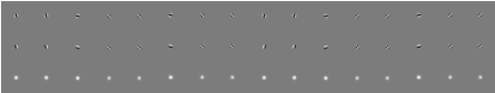
The 32 wavelets related to the 2-D double-density dual-tree complex DWT are illustrated in Figure 8 as gray scale images. The wavelets here are oriented in the same directions as those of the real DWT version; however, here we have two in each direction. We can interpret the first row of wavelets at the real part of a set of sixteen complex wavelets and the second row as the imaginary part. Then, the third row represents the magnitude of the sixteen complex wavelets. As you can see, the magnitudes form sixteen bell-shaped envelops without any oscillatory behavior. We plot these wavelets using the following MATLAB code.

>> J = 4;
>> L = 8*2^(J+1);
>> N = L/2^J;
>> [Faf, Fsf] = FSdoubledualfilt;
>> [af, sf] = doubledualfilt;
>> x = zeros(2*L,16*L);
>> w = cplxdoubledual_f2D(x, J, Faf, af);
>> w{J}{1}{1}{1}(N/2,N/2+0*N) = 1;
>> w{J}{1}{1}{2}(N/2,N/2+1*N) = 1;
>> w{J}{1}{1}{3}(N/2,N/2+2*N) = 1;
>> w{J}{1}{1}{4}(N/2,N/2+3*N) = 1;
>> w{J}{1}{1}{5}(N/2,N/2+4*N) = 1;
>> w{J}{1}{1}{6}(N/2,N/2+5*N) = 1;
>> w{J}{1}{1}{7}(N/2,N/2+6*N) = 1;
>> w{J}{1}{1}{8}(N/2,N/2+7*N) = 1;
>> w{J}{1}{2}{1}(N/2,N/2+8*N) = 1;
>> w{J}{1}{2}{2}(N/2,N/2+9*N) = 1;
>> w{J}{1}{2}{3}(N/2,N/2+10*N) = 1;
>> w{J}{1}{2}{4}(N/2,N/2+11*N) = 1;
>> w{J}{1}{2}{5}(N/2,N/2+12*N) = 1;
>> w{J}{1}{2}{6}(N/2,N/2+13*N) = 1;
>> w{J}{1}{2}{7}(N/2,N/2+14*N) = 1;
>> w{J}{1}{2}{8}(N/2,N/2+15*N) = 1;
>> w{J}{2}{1}{1}(N/2+N,N/2+0*N) = 1;
>> w{J}{2}{1}{2}(N/2+N,N/2+1*N) = 1;
>> w{J}{2}{1}{3}(N/2+N,N/2+2*N) = 1;
>> w{J}{2}{1}{4}(N/2+N,N/2+3*N) = 1;
>> w{J}{2}{1}{5}(N/2+N,N/2+4*N) = 1;
>> w{J}{2}{1}{6}(N/2+N,N/2+5*N) = 1;
>> w{J}{2}{1}{7}(N/2+N,N/2+6*N) = 1;
>> w{J}{2}{1}{8}(N/2+N,N/2+7*N) = 1;
>> w{J}{2}{2}{1}(N/2+N,N/2+8*N) = 1;
>> w{J}{2}{2}{2}(N/2+N,N/2+9*N) = 1;
>> w{J}{2}{2}{3}(N/2+N,N/2+10*N) = 1;
>> w{J}{2}{2}{4}(N/2+N,N/2+11*N) = 1;
>> w{J}{2}{2}{5}(N/2+N,N/2+12*N) = 1;
>> w{J}{2}{2}{6}(N/2+N,N/2+13*N) = 1;
>> w{J}{2}{2}{7}(N/2+N,N/2+14*N) = 1;
>> w{J}{2}{2}{8}(N/2+N,N/2+15*N) = 1;
>> y = cplxdoubledual_i2D(w, J, Fsf, sf);
>> y = [y; sqrt(y(1:L,:).^2+y(L+[1:L],:).^2)];
>> figure(1)
>> clf
>> imagesc(y);
>> title('Complex 2-D Double-Density Dual-Tree Wavelets')
>> axis image
>> axis off
>> colormap(gray(128))

In this program, all of the wavelet coefficients are set to zero, for the exception of one wavelet coefficient in each of the sixteen subbands. We then take the inverse wavelet transform. This code produces the following gray scale image:

Figure 12.   Complex 2-D Double-Density Dual-Tree Wavelets.

Summary of Programs:

1. FSdoubledualfilt.m - Set of filters for the first stage
2. doubledualfilt.m - Set of filters for the remaining stages
3. afb3_2D.m - 2-D analysis filter bank
4. sfb3_2D.m - 2-D synthesis filter bank
5. doubledualtree_f2D.m - Forward 2-D real double-density dual-tree complex wavelet transform
6. doubledualtree_i2D.m - Inverse 2-D real double-density dual-tree complex wavelet transform
7. cplxdoubledual_f2D.m - Forward 2-D complex double-density dual-tree wavelet transform
8. cplxdoubledual_i2D.m - Inverse 2-D complex double-density dual-tree wavelet transform
9. cshift2D.m - Circular shift